The world we are in is very automated

In the world we are in, automation is becoming increasingly common. It is impossible to go about your day-to-day life without some sort of automated decision-making occurring. Some are minor (e.g. what YouTube video is recommended), but others may be life-changing (e.g. a home loan application being rejected).

Regardless of the size of the decision, as humans we are wired to need to rationalise all decision-making. That is, why the decision was made is as important (or even more important than what decision was made).

In this blog post, I will explore why machine learning explainability is important, as well as some techniques in making machine learning models more explainable. In some circles, this is also known as Explainable Artificial Intelligence (XAI).

As IBM puts it:

Explainable AI is used to describe an AI model, its expected impact and potential biases. It helps characterize model accuracy, fairness, transparency and outcomes in AI-powered decision making. Explainable AI is crucial for an organization in building trust and confidence when putting AI models into production.

It is crucial for an organization to have a full understanding of the AI decision-making processes with model monitoring and accountability of AI and not to trust them blindly

Image from Pixabay

Why do we need to explain ML models?

There are a few reasons why explainability is crucial and I cover a few below:

1. It is the Law!

This requirement for explaining automated decision-making is also rooted in law. Under the European Union General Data Protection Regulations (EU GDPR), it provides that a person in the EU can request for reasons for decisions from an automated decision-making system. Furthermore, in specific industries (e.g. finance and healthcare), explainability ensures that decision-making is not discriminatory or illegal. For example, an automated home loan application approval process cannot consider things like culture or race when making a decision.

2. Salvaging a White Elephant

In some cases, significant resources and money made have been spent on developing a predictive model. To achieve high accuracy, a complex, but highly accurate model is created. These models may use neural networks/deep learning or other complex algorithms.

While neural networks can potentially yield very accurate predictions, their explainability is inherently quite lacking. It is difficult to easily say “the model got this result because of XYZ” due to the nature of deep learning - the word ‘deep’ itself implies that the hidden layers are, well, hidden!

Without explainability, the model can’t provide insights because simply providing a prediction. It also makes extensibility and maintenance a nightmare. Furthermore, as mentioned above, it may be illegal, as it doesn’t meet the audit and transparency requirements under industry regulation! This means that a lot of money was spent on a white elephant project.

When faced with such a dilemma, there are generally two options:

1. Scrap this model and go back to a more basic model (e.g. rules-based one). However, this will mean years of work and money is thrown away!
2. Create an interpretability model on top of the complex model that helps ‘explains’ what the model is doing

Obviously option two is more appealing and makes most sense. It also complies with a software engineering concept of extensibility - you should extend existing functionality, not replace it. In this case, this extension is a ‘black-box’ approach (literally) because you have no idea what the original model is doing under the hood.

This is probably not how you should do machine learning… Image from XKCD

3. Machine learning is part of a larger predictive system

Solely doing decision-making on an entirely automated system presents inherent risks. Therefore, as part of many hybrid and ensemble models, often different types of algorithms and rules-based modelling are combined together - different angles of approaching the same problem will yield better coverage. If you are interested in how hybrid models works, check out my prior blog post, which goes into more detail.

When the machine learning component is just middleware or an intermediate step, having explainable results is very crucial. This is because the why is just as important as the prediction, and often the explainability factors are fed into the downstream model.

Here is a simple example - there is a spam detection system with three parts:

• Disallow list component (i.e. checks whether the email is from a disallowed email address and if so, block)
• Machine Learning component that classifies incoming email as spam vs not-spam
• Risk rules (rules-based) that are specific to certain industries (e.g. for finance emails, block everything with the word ‘Crypto’ in it)

In the above, ideally you want the ML component to provide:

• The prediction/classification - i.e. spam vs not-spam
• Main factor for its classification - e.g. email subject is suspicious, Email address is suspicious

This is so in the risk rules step, you can create risk rules revolving around the classification - e.g. where the email address is suspicious and it is a disallowed email address, the risk is High. If the email subject is suspicious only, it may be Medium.

4. Window into the ‘soul’ of the model

Machine learning models are analogous to naive chidren - they don’t have much context of the world, so most of their decision making is based solely on the inputs that you provide them. Adult humans generally have more context and experience of the world, so it is often easy for this to creep into the way we perceive/analyse a ML model’s prediction.

That is, we assume there is a ‘common sense’ or grounded reason to arrive at a prediction (when in fact they haven’t).

Two cautionary tales circulate in the machine learning community that illustrate this fact: one one about camouflage tanks and one about huskies!

The camouflage tank story goes as follows: the US Army wanted to create a neural network to automatically detect camouflaged tanks. Researchers then fed the algorithm images of camouflaged tanks and non-camouflaged tanks and were surprised the algorithm was performing extremely well!

Excited with the results, they enlarged the project to test it against more images - this resulted in the algorithm tanking (pardon the pun) in its performance. Then they realised that all the images of camouflaged tanks were under a cloudy sky. So what they had achieved was an algorithm that was excellent at telling whether the sky was dark or not.

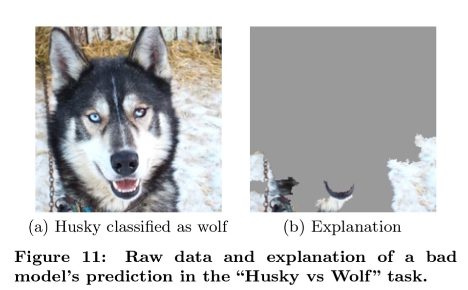
Similarly, a project attempted to create a model that could classify images between wolves vs dogs. Again, they achieved a remarkably high accuracy and were stunned, followed by the performance tanking when exposed to more images.

Then, again, they realised that all the images of wolves were in snow, while the images of dogs were not. So what they had created was an excellent classifier of snow vs non-snow!

Good engineering - good cogs Image from “Why Should I Trust You?” Explaining the Predictions of Any Classifier

Both these cautionary tales highlight a very important point: how the model arrives at a decision is just as important as what the decision is! In particular, what data points did the model consider to make its decision?

There are real-life examples of this occurring which have real-life implications. I’ve covered bias in another blog post, but to briefly recap, biased datasets result in biased models.

Interpretability is therefore crucial in understanding the factors that are used in the model.

Examples include:

• Using the CV of existing successful C-level executives to train an algorithm on what characteristics constitute a ‘successful candidate’. However, due to historical gender and cultural bias, the majority of C-level executives in the past are generally male and of a certain culture (depending where you are). The result is the algorithm perpetuates and further enhances this bias in predictions.
• A massive blind spot in a self-driving car algorithm, which only occurs 0.1% of the time but results in fatal accidents.

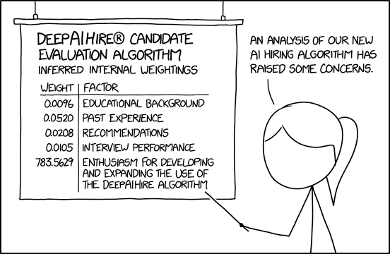When the hiring AI goes wrong… Image from XKCD

A good way to expose blind spots and bias in models using sensitivity analysis and random data points to see how the model reacts. For example, if you trained a model on a dataset where the maximum income of a person was $500,000, see what happens if you make it $20 million. This will expose how sensitive the model is to that variable and also whether it is correctly factoring it in as intended. For example, if a home loan approval model doesn’t even care about the person’s income, it is likely biased by something even greater (e.g. the person’s job, age, culture).

What types of interpretability can you have?

Before we dive into the how - I’ll first explain the types of interpretability. At a high-level, interpretability can be broken up into:

• Global interpretability vs local interpretability
• Model-agnostic vs model-specific interpretability
• Post-hoc explanation vs intrinsic explanation

Global interpretability focuses on explaining the decisions of the model in general (or as a whole), whereas local interpretability focuses on explaining each specific prediction/decision. Both are important - you want to know how the model performs in general, but also be able to explain each decision.

Interpretability can also be categorised between model-agnostic vs model-specific methods. Model-agnostic are ways of explaining models which can be used for many different types of models - focusing on the input and output of the model. Model-specific, on the other hand, is suitable and designed by a particular type of model (e.g. tree-based, neural network, etc.), so is more closely linked to the structure of the algorithm.

An example of a model-specific are saliency maps, which specifically are designed to explain image recognition models. I won’t cover this in detail for this blog, but because is an example of it working.

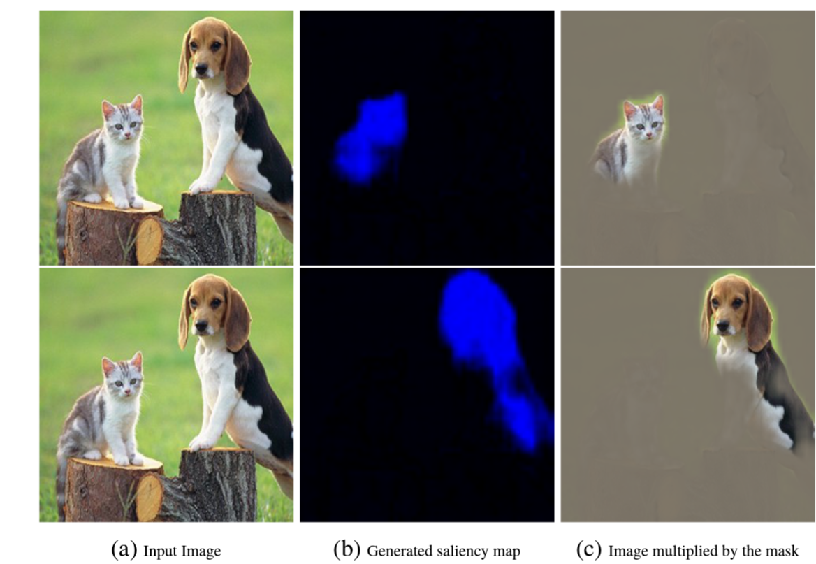Saliency maps show which pixels the model considered most relevant when identifying the cat and dog Image from Real Time Image Saliency for Black Box Classifiers

A post-hoc explanation is an attempt to explain how the model arrived at a decision after the prediction/training is made (by focusing on the inputs and outputs). Because it focuses on the inputs and outputs, post-hoc explanations take a black-box approach and only can provide an approximation of what the model is actually doing.

In contrast, intrinsic explanations are generally algorithms which inherently provide a certain degree of explainability. For example, tree-based algorithms can generally show what points they used to arrive at a prediction.

Also see Google’s own explanation of the different ways to interpret a ML model.

I will now discuss LIME - one of the most popular methods to XAI.

Locally Interpretable Model-Agnostic Explanations (LIME)

LIME is a popular local, model-agnostic and post-hoc explanation method to model interpretability. The core concept of LIME focuses on two points:

• humans are inherently better at interpreting simpler models (e.g. linear and models)
• Complex ML models are ‘black boxes’ with a known set of inputs (i.e. datasets) and outputs (i.e. predictions)

Therefore, what LIME does is create a surrogate model (i.e. a model that sits on top of the existing model), which approximates the underlying complex model’s behaviour.

The way this is done is by creating a linear model through deliberately tweak the inputs to see how the underlying model’s output changes (i.e. perturbations).

Explanation of how LIME works in a nutshell Image from “Why Should I Trust You?” Explaining the Predictions of Any ClassifierE

LIME:

• focuses on local interpretability in the sense that the model attempts to explain/approximate the individual predictions of the underlying model.

• model-agnostic, LIME can explain most types of ML models. It is generally a cost-effective way to retrofit interpretability into a model. Analogously, it is like adding a speedometer to a bicycle to let the cyclist know how fast it’s going!

• Being a linear model, it can self-assess how trustworthy/accurate its approximation is (by way of goodness-of-fit statistics). That is, the better the fit, the better the surrogate model is at explaining the underlying model.

• stability/consistency of the underlying model can be tested - consistency is important, as if explanations are not stable when there are only minor changes to input data:

  • the underlying model may not be particularly accurate/good, or
  • the explanation is not particularly good

LIME supports multiple types of ML models:

1. For tabular features - weighted combination of columns
2. For textual features - the presence/absence of words
3. For image features - the presence/absence of pixels

For example, below is a simple example of LIME interpreting a column-based model:

from lime.tabular import LimeTabularExplainer

# Create your model here
# create model etc.

explainer = LimeTabularExplainer(
    training_data=df_train.drop('target'),  
    mode='classification',
    training_labels=df_train['target'],
    feature_names=model.feature_name()
)

# Now explain a particular prediction
i=12 # Let's pick 12

explainer.explain_instance(
    data_row=df_predict['target'][i], 
    predict_fn=model.predict,
    num_features=5 # Max number of features explained
)

However, the greatest pitfall with LIME is, being a linear model, if the underlying model is significantly non-linear, then LIME’s explanation would only be a ‘best guess’ essentially. That is, not all relationships can be easily explained via linear models.

LIME also doesn’t consider the context of the problem. For example, imagine you have an underlying model which predicts the price of a house. Without sufficient context, LIME may explain that if the land size = 0, then the price is $X. However, in the context of the real world, if the land size = 0, the house price should = $0.

Next up, global interpretability!

Global Interpretability - Partial Dependence Plots

Global interpretability, unlike local interpretability, aims to describe the average behaviour of a ML model. Global intepretability focuses on expected values based on the distribution of the input and output data.

As Kaggle puts it:

While feature importance shows what variables most affect predictions, partial dependence plots show how a feature affects predictions.

The most common method is via Partial Dependence Plots (PDP). PDPs depict the functional relationship between certain input variables and the model output. For example, the below PDPs show how certain features relate to the Californian housing price.

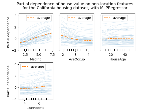Example of PDPs - the orange line is the ‘average behaviour’ Image from Scikit-Learn

In particular, it shows the type of relationship as well (e.g. linear, curvilinear, step, no-linear).

PDPs are a good way of ‘sanity checking’ a model to see whether some features are skewering the model output, or even whether certain features are even used at all.

Explaining Tree-based Algorithms

The next section will focus on model-specific interpretability - in particular, focusing on tree-based algorithms.

The reason tree-based algorithms are selected is because due to the intuitive nature of decision trees, they come with mechanisms that are easier to understand by humans.

The two I’ll cover are feature importance and SHAP.

Feature Importance using XGBoost

XGBoost is a popular tree-based algorithm that is increasing in popularity due to its explainability and effectiveness. The algorithm will generate multiple trees iteratively and use optimization/boosting to eventually create the best tree.

Broadly, there are two main metrics in measuring how feature importance. Feature importance essentially shows how much a feature affects the prediction. either by:

• Gain - the relative contribution of the feature to each tree
• Cover - broadly, the relative number of times this feature shows up in trees (as a %)
• Weight - the number of times the feature appears in trees

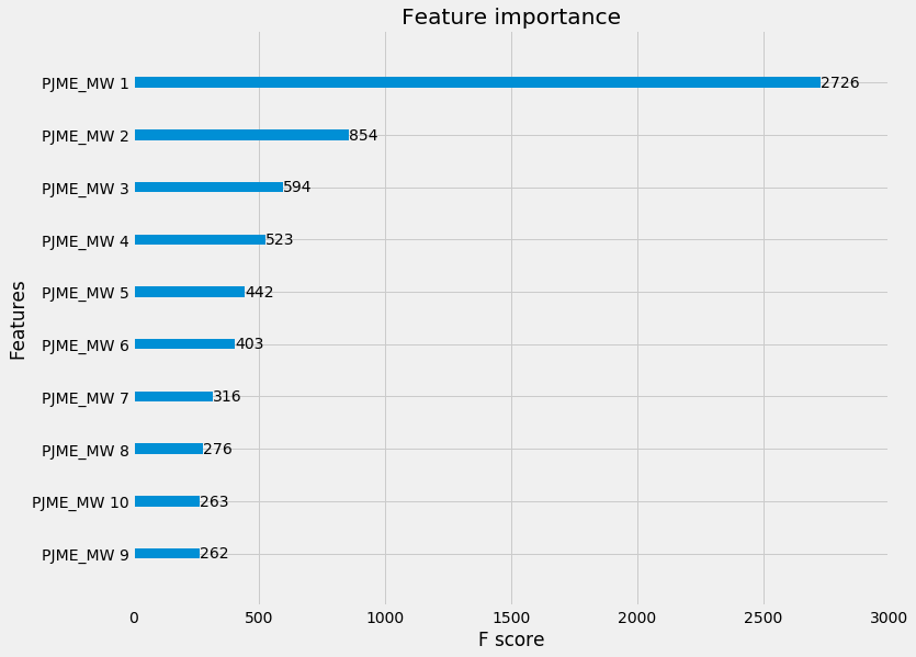An example from my prior blog post - you can see that for this forecasting model, the ‘PJME_MW_1’ feature contributed the most to the models

However, the shortcomings of relying just on feature importance alone is it doesn’t compare multiple models and what would happen if the feature was removed. That is, consistency of feature importance across multiple models is important - i.e. if we tweak the model to rely on a feature even more, you should see the feature importance go up. If not, it is inconsistent and the feature importance metric is not reliable.

One way to address this shortcoming is through SHAP.

SHapley Additive exPlanations (SHAP)

SHAP uses cooperative game theory to model how the ‘players’ (i.e. features) ‘contribute’ to the outcome of the game (i.e. the model’s predictions). It will remove features and see the impact to the model’s predictions - i.e. if a ‘player’ contributes more to the outcome, the outcome will be more affected when they are removed.

SHAP values are expressed based on a particular baseline/expected value Values can be negative (i.e. reduce the output value below the baseline value) or positive (i.e. increase the output value above the baseline). The baseline value is generally the average of all predictions.

Example of SHAPley values Image from Measuring Impacts of Urban Environmental Elements on Housing Prices Based on Multisource Data — A Case Study of Shanghai, China

For example, the above is an explanation of a model that predicts prices of mansions in Shanghai, China. The baseline prediction is ¥59,000/m2 (the figures are expressed in 10,000 units). You can then see:

• features that increased the predicted value are in pink, where the larger the bar the more it contributed. In this case, the largest contributor is EC_DIS (i.e. distance to the city employment centers)
• features that decreased the predicted value are in blue (i.e. the age of the mansion was the largest contributor)

There are also other ways to visualise SHAPley values as well, such as bar plots and beeswarm plots:

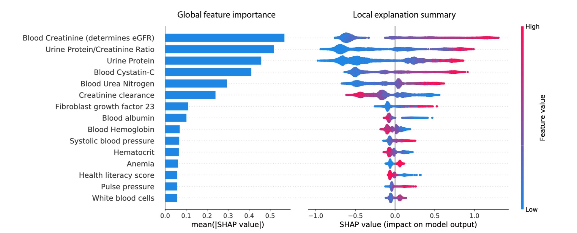Examples of bar plot and beeswarm plot Image from Explainable AI for Trees: From Local Explanations to Global Understanding

You can see the bar plot is more of a summary (generally the mean absolute value), while the beeswarm plot shows more detail on how each feature affects the model output (by showing the entire distribution, rather than just the mean absolute value).

There are more visualisations and more explanations in the official documentation.

Below is a small example of how easy it is to use SHAP:

import pandas as pd
import shap
import sklearn

# Do preprocessing etc. 
# to get training dataset and target/labels
df_train = ### Dataframe output from pipeline

# Do your regular ML training cycle here 
# For example - L1/L2 linear regression model
model = sklearn.linear.model.ElasticNet()
X = df_train.drop('target')
y = df_train['target']
model.fit(X, y)

# Now you can explain it using SHAP
explainer = shap.Explainer(
    model.predict,
    shap.utils.sample(X, 1000) # 1000 instances
)

shap_values = explainer(X)

# If you want to see a waterfall visualisation
shap.plots.waterfall(
    shap_values, 
    max_display=20 # max no. of features to plot
)

# If you want to see a bar chart visualisation
shap.plots.bar(shap_values)

Why is SHAP so powerful?

SHAP is a powerful method of explaining ML models because of its intuitive nature. Using ‘contributions’ rather than a linear model means it is able to explain tree-based models better (rather than trying to fit a surrogate linear/logistic model, like what LIME does). It’s flexiblity has now extended to include KernelExplainer() and DeepExplainer(), each dealing with kernel-based algorithms (e.g. K-nearest neighbour) and neural networks respectively.

It also is can do both global and local interpretability - SHAP values explain how the models’ features generally contribute to the prediction. Likewise, it can also explain specific predictions, or even a random sample of the predictions (like in the example above).

Closing Thoughts

We’ve explored the importance of explaining ML models, as well as some of the methods to do so. Hopefully this blog post will inspire you to continue your research and start applying it to your own ML modelling!