Why is Feature Engineering and Heuristics so important?
The way Google approaches ML engineering is building a good machine learning system requires good engineering. In Google’s words:
…most of the problems you will face are, in fact, engineering problems. Even with all the resources of a great machine learning expert, most of the gains come from great features, not great machine learning algorithms.
Feature engineering is the process of adding, modifying and removing data into your dataset so it is optimised for machine learning. Essentially, training a ML is like teaching a kid - you need to put in the effort to make good teaching materials and examples if you want the kid to learn how to think and come up with good general and logical rules.
That is, good features produce more flexible and easy to understand models.
Furthermore, a common mistake made by many people is assuming that machine learning will solve all your problems. However, as humans, we generally have implemented and documented many years of built-up knowledge in pre-existing rules. So why not leverage these existing rules in your model?
In this blog post, I’ll explore how you can use both feature engineering and rules-based modelling to greatly boost the performance of you machine learning model.
 Good engineering - good cogs
Image by Arek Socha from Pixabay
Good engineering - good cogs
Image by Arek Socha from Pixabay
- Why is Feature Engineering and Heuristics so important?
- Feature Engineering and Heuristics
- Documenting your features and deleting unused/legacy features
- Generating new features out of existing data and observations
- Start with direct features and then move onto ‘learned’ features
- Feature Selection and Dimension Reductionality
- ‘Non-ML’ components make up the majority of a ML system
- Delta Testing - the regression test for ML systems
- Closing Thoughts
Feature Engineering and Heuristics
In a nutshell, feature engineering involves:
-
Feature selection and elimination - picking which features you want to keep and use to train the model, excluding the ones that supposedly affect the outcome the least.
-
Feature extraction - adding in new features based on domain knowledge and knowledge of the dataset (e.g. adding in public holiday dates for a time series forecasting)
Since ML is solving an existing problem where you likely already have some form of rules-based approach (e.g. treat email as spam if it’s from a blacklisted email address), you can harness these rules by converting them into features. Google refers to this as ‘lifting’ your ML model with these rules.
Another term for rules is heuristics, which are also commonly known as ‘rule of thumb’. A rules-based model (a.k.a. heuristics-based modelling) reflects the current business processes or based on a set of rules. For example, a rules-based fraud detection system could be as simple as:
- If IP address from certain geographic region -> Alert
- If IP address from blacklist -> Block
- If connection has excessively high traffic -> Block
- If multiple connections are made within a 5 minute window -> Alert
Many of these rules may be derived from years of business experience and known practices already adopted. This makes sense, given the goal of a machine learning model is to improve existing processes.
However, there is a trade-off point where ML becomes better than a complex unmaintainable rules-based model. If you need to pick between a very complex and interlocking heuristics model vs a ML model, it is recommend you pick ML as it is easier to update and maintain.
The balancing act is adding enough heuristics into your ML algorithm, but not overly complicate it. This hybrid approach of heuristics plus machine learning is very powerful and is essentially an extension on feature engineering. As shown below, most of the incorporation of heuristics involves generating new features of some kind.
 Know the Rules
Image by Gerd Altmann from Pixabay
Know the Rules
Image by Gerd Altmann from Pixabay
Bad Features means bad models
Machine learning algorithms are trained over a dataset and therefore having very large datasets without feature engineering means:
-
Much slower training times due to higher processing power required
-
Curse of dimensionality - the more features in a dataset, the more complex the model and therefore more likely overfit will occur
-
‘Rubbish’ and ‘noisy’ data points may distort/skewer the results
-
Some data might not be suitable for some predictive models (e.g. using race, religion to profile people)
Generally speaking, throwing all your data at the machine learning algorithm will not yield the best results. Even when you use services such as automated machine learning (AutoML), the system will apply feature engineering first - it won’t just throw all the data at every algorithm and expect an answer!
Hybrid Approach - a great place to combine feature engineering and heuristics
A great starting place in feature engineering is leveraging all those existing heuristics you have built up.
Google has an excellent guide on Machine Learning Engineering Best Practices that I highly recommend you read.
Some of the methods Google recommend you incorporate heuristics into a ML model include:
-
Preprocess using the heuristic - e.g. in the above example where you already have a blacklisted email list, simply exclude everything in the blacklist as part of preprocessing. No need to reinvent the wheel on what ‘blacklist’ means.
-
Create a feature directly based off the heuristic - e.g. in the above example where you already have a blacklisted email list, simply add a new feature which is Y/N flag whether its in the existing blacklist
-
Mine the raw inputs of the heuristic. However, Google recommends that as a general rule, you should either take the input of the heuristics or the output of applying the rules, but don’t do both.
-
Modify the target variable - this is in instances where the heuristic captures some information not currently contained in the target variable. Google gives an example of adjusting the target variable (number of downloads) by multiplying with the result of a heuristic calculating average rating. In the above example, without the adjustment, the algorithm may favour garbage apps with high number of downloads.
The end result may be that a hybrid model with 90% rules-based and 10% machine learning will outperform any 100% machine learning model.
Leveraging the power of ‘classical’ rules-based models
There are other forms of rules-based models that have existed in certain industries for many years which are ‘tried and proven’. While they may not form as well as a very well built-in ML system, it is a great starting point to understand the business context.
Other types of rules-based analysis that are tried and proven:
-
Recency-Frequency-Monetary (RFM) model to target marketing/advertising on existing customers
-
Moving Average (MA) model for forecasting and the Moving Average Convergence/ Divergence (MACD) method for algorithmic trading
-
Popularity-based Recommender Systems - recommend to customers the most popular/best-selling item
Documenting your features and deleting unused/legacy features
Google ML Engineering Best Practices mentions that documenting features is an important step. This helps with feature lifecycle management and deleting legacy/unused features. In particular you should document:
- Creator/owner
- What the feature is
- Where the feature came from
- How is the feature relevant
- What are the possible valid data points in the feature (e.g. list of countries)
Unused features ultimately create technical debt and a good feature lifecycle policy will delete them out. That is, if you aren’t using it, drop it!
Google’s tip in deciding whether to keep a feature - coverage, which is how many examples/rows are covered by the feature? For example, if the feature only is applicable to 2% of the rows, then it’s not going to be very effective. Also remember to consider the coverage within a sub-group - for example, if a feature only relates to 1% of the customers that are VIP but is very accurate at predicting 90% of these VIPs, then it may be a feature worth keeping.
Furthermore, make sure your features are version controlled and have auto-incrementing timestamp hashed versions.
Generating new features out of existing data and observations
A good starting place for feature engineering is to generate features out of existing features. I’ll cover two techniques that can be used:
-
Binning and Discretization
-
Crosses
Binning/Discretization consists of taking a continuous feature and creating many discrete features from it. Consider a continuous feature such as age. You can create a feature which is 1 when age is less than 18, another feature which is 1 when age is between 18 and 35, et cetera. Don’t overthink the boundaries of these histograms: basic quantiles will give you most of the impact. Turning continous variables that are skewered into discrete variables
There are two mains to bin a continuous variable - bin them into ‘buckets’ of equal width or bin them into ‘buckets’ of equal frequency. For example:
- Equal width - bucket the ‘Age’ column into 10-20, 21-30, 31-40, 41-50
- Equal frequency - bucket the ‘Age’ column so each bucket is same size, such as 10-17, 18-35, 36-99
Equal width binning does not improve spread of data but does handle outliers, as it’ll show up in the first or last bucket. On the other hand, equal frequency improves value spread, but you no longer capture the original spread of your data.
Binning also works to reduce the number of categories you have in a feature - e.g. only keep Top 10 features as it is and group all the rest together. For example, region of movie produced could be: USA, UK, Germany, Other.
 Buckets
Image by S. Hermann & F. Richter from Pixabay
Buckets
Image by S. Hermann & F. Richter from Pixabay
Crosses combine two or more features to generate a new column. For example, if you have Male/Female in one column and country in another column, your new feature could be: {male, Canada}, {female, Canada}, {male, USA}, {female, USA}. Where some categories have 3 or more potential classes, crossing is computationally expensive and may result in overfit.
Use Specific Features where possible
Google also recommends to use very specific features when you can. With tons of data, it is simpler to learn millions of simple features than a few complex features.
Counter-intuitively, this may generate a lot more features, where each feature only covers a small set of your data, but all these extra features have an overall coverage of 90%+ of your data. Because of the way ML algorithms train, this method may deliver better results than a simple overly complex features with no obvious/discernable pattern.
Also remember that you can use regularization to eliminate low-value features that don’t apply to most of the dataset.
Generate new features out of observed errors
If you have say a classification model, you can review your false positives and negatives to see why the model was ‘wrong’. For example, it could be those customers had invalid contracts or already transferred out. You therefore could generate a new feature (IsValidContract_YN) which calculates whether a contract is valid based on its start and end date.
Start with direct features and then move onto ‘learned’ features
Some algorithms actually will generate/’learn’ new features out of an existing dataset, generally by way of an unsupervised learning algorithm. Examples of this include FeatureTools, an open-source Python library that automatically generates hundreds of new features from your existing features.
Another example is K-means clustering - this algorithm clusters the dataset into a pre-specified of groups (K) by essentially using the ‘distance’ between the data points. K-Means is an unsupervised machine learning algorithm. You can then add the cluster group as a feature (or only use the cluster group as a feature and remove the remaining features).
Google actually recommends you only start including these ‘learned’ features after you have established a baseline model. That is, don’t introduce these features until you’ve done your first model. The reason is you have an extra layer of complexity - now the generation of the features itself is another model you need to tweak and maintain.
Feature Selection and Dimension Reductionality
Feature selection is a key aspect of feature engineering is removing unnecessary and noisy features. Like a crowded and noisy bar, it is difficult to get meaningful insight if there is a lot of noise.
There are two main methods of feature selection that are used: Filter methods and Wrapper methods.
I’ll explain both in detail below, but as a primer, a comparison of both in a nutshell is as follows:
| Filter | Wrapper | |
|---|---|---|
| Process | Non-iterative | Iterative |
| Computation Speed and Resource | Fast and Low | Slow and High |
| Metric to optimise and evaluate | Statistical tests - feature vs target | Model feature importance |
| Scalability - i.e. adding more features | Much higher | Much lower |
| Ability to Identify Optimal Features | Lower - tends to overfit as well | Higher - lower tendency to overfit as well |
Filter Methods
Filter methodologies use statistical measures to score the correlation or dependence between features and the target variable. The lowest scoring features are then filtered out from the training dataset. It is a simple and effective way to identify irrelevant/redundant features without high computation/resourcing.
The typical Filter Method process is non-iterative, meaning once the features are selected, the model is trained once on that particular set of features:
- Select all Features
- Filter out Features using Stats tests
- Train ML Model
- Evaluate ML Performance
Common ‘filter’ methods include:
-
Cardinality and Missing Data Thresholds - filter out features with a high percentage of missing values or with little or no variation (e.g. 99% of data is ‘Yes’)
-
Bivariate screening - algorithms used to assist in determining which features have the biggest effect on the target. These algorithms produce a statistical measure that can be used to compare the correlation, relationship or dependence between two variables. You can then select the ones which have the highest number.
-
Dimension reductionality algorithms - these algorithms main to reduce the a very high number of features into a smaller set that retains most of the information from the original dataset.
-
Feature Agglomeration/clustering - these algorithms aim to cluster features together based on related they are with each other. Unlike bivariate screening which focuses on relationships between features vs targets, feature clustering focuses on relationships between features.
I’ll now discuss these into a bit more detail below.
 Image by Hugo Hercer from Pixabay
Bivariate Statistical Tests
Google’s approach is there are angles of statistical analysis:
-
Descriptive - univariate analysis because they only focus on one feature (e.g. median of ‘Age’, number of missing rows in ‘Height’)
-
Correlative - bivariate analysis as it looks a the relationship between a feature vs target
-
Contextual - analysis of the features in a context, mainly time-based (e.g. number of observations over a period of time) and agent-based (e.g. number of transactions by a user ID)
For the purposes of this section, we’ll only focus on bivariate statistical tests.
For reference, the type of algorithm used depends on the data type:
| Feature Type | Target Type | Recommended Algorithm |
|---|---|---|
| Numerical | Numerical | Pearson Correlation Coefficient |
| Numerical | Categorical | ANOVA statistical test |
| Categorical | Numerical | One-Way ANOVA F-test |
| Categorical | Categorical | Chi-Squared Test |
Pearson’s Correlation Coefficient calculates the correlation between two variables (as expected earlier). The correlation will be between -100 to 100%. The further away from 0, the greater the relationship.
One-Way ANOVA F-test is a statistical test to determine whether the means of two variables are the same. It is used for categorical features vs numerical target (hence why it is ‘one-way’, as it can’t be used backwards). One-Way ANOVA produces a F-score - the higher the number, the greater the relationship.
Pearson’s Chi-squared test is a statistical test to determine whether a variable is dependent/independent of another variable.
Chi-Squared produces a chi-squared distribution - the higher the number, the greater the relationship.
LDA, ANOVA and Chi-Squared are statistical tests that require first assuming there is no dependence (ie the null hypothesis) and calculating whether this is rejected:
| Statistical Test | Null Hypothesis default position unless prove otherwise |
Alternative Hypothesis need statistical evidence to prove correct |
|---|---|---|
| Hypotheses | The variables are independent (i.e. not dependent on each other). | The variables are dependent on each other. |
| P-Value | Greater than 0.05 | Less than 0.05 |
| What P-Value means | There is no statistical evidence the variables are dependent. Null hypothesis is not rejected. |
There is statistical evidence the variables are dependent. Null hypothesis is rejected. Furthermore, there is only a 5% chance this was incorrect proven by chance. |
Note that because it only compares two variables at a time, it may over-simplify the feature selection process and the results of these should be taken with a grain of salt. These are generally used when there is a very large amount of features (e.g. over 500) and it is too computationally expensive to do RFE on all the variables at a time or when PCA isn’t appropriate.
In general, the focus should still be on whether the model as a whole is more accurate with the inclusion/exclusion of particular variables.
Dimension Reductionality Algorithms
Dimension reductionality is commonly done by three algorithms:
-
Principal Component Analysis (PCA)
-
Linear Discrimiant Analysis (LDA)
-
t-Distributed Stochastic Neighbor Embedding (t-SNE)
PCA, LDA and t-SNE are complex algorithms which all aim to do one thing - reduce a larger group of features into a smaller dataset that tries to capture as much of the original information as possible. In a technical sense, it looks for linear combinations of variables which best explain the data.
The way each one does it have different focuses:
-
PCA aims to retain as much of the covariance (i.e. correlation) between features as possible. In contrast, LDA aims to retain as much of the differences between features as possible
-
PCA is an unsupervised learning algorithm (which doesn’t require labels). In contrast, LDA is a supervised learning algorithm as the target needs to have class labels.
-
t-SNE is a manifold learning algorithm, which aims to visualise datasets with a lot of dimensions (e.g. in image recognition and NLP) - it aims to reduce features to only 2 or 3 so it can be easily visualised.
-
LDA limit the maximum number of features produced, while PCA does not.
-
t-SNE in contrast has a maximum feature size of up to 50 features. A good trick is to use LDA first to reduce to 50 then use T-SNE.
-
LDA is useful for multi-class classification - i.e. your target variable has 2 or more potential classes.
-
LDA requires a minimum sample size - size must be greater than number of features (e.g. if you have 300 features, you need at least 300 rows).
-
As PCA is aiming to retain as much of the covariance between features, it assumes a linear relationships of correlation between variables. If you want to capture non-linear correlations, you will need to use kernel PCA (kPCA) and apply a different relationship (e.g. polynomial kernel). In contrast, t-SNE does not have this assumption.
-
PCA will endeavour to reduce the features into principal components (PC) which uses a linear-based method to capture the most amount of the features’ variances. That is, we’re trying to project a straight line on the ‘direction’ which explains the most amount of variance (i.e. most spread out) of all the features. The ‘direction’ is measured in eigenvectors (e.g. 45 degrees vector) and the amount of variance on the PC is measured by eigenvalues.
-
The 1st PC will be the eigenvector that has the highest eigenvalue (i.e. the direction that explains the most amount of variance of all the features). The 2nd PC will have the 2nd highest eigenvalue etc. The result of PCA is features with higher variances are more likely to have their co-variance kept by the PC compared to features with lower variance. i.e. features that don’t have any variance probably aren’t that important - almost like a static noise in the background.
-
Analogously, if each feature was a group of people spread out in a room (i.e. Group A people, Group B people), each PC is a snapshot photo that tries to get as many people from each group as possible. You take the photo from different angles and you get different snapshots. Invariably, groups with the most spread out people will have a higher chance of ending up in the photos.
-
PCA requires a pre-determined cut-off of how much co-variance you want to explain. For example, if you set a 99% co-variance cut-off, you might use 136 PCs to explain 330 features. If it is 95%, it may be 48 PCs to explain 330 features.
All these algorithms reduce dimensionality at the sacrifice of clarity. Furthermore, the original features are no longer retained so model interpretability is more difficult. That is, it is more difficult to explain which of the original features contributed to the prediction and how they did.
 Image by Steve Johnson from Pexels
Feature Agglomeration (i.e. feature clustering)
Feature agglomerations aims to identify multicollinearity - that is, the amount of correlation between features. Unlike bivariate screening described above which focused on the relationship between the features and the target, feature agglomeration focuses on the relationships between features.
If two features have a perfect correlation, they also have perfect collinearity. A change in one of the collinear features affects the other feature.
In general, the higher the multicollineraity, the more difficult it is to model the data. This is because the relationships between features wreck havoc on many algorithms - e.g. linear regression generally does not work with high multicollinear datasets. It is difficult to determine the relationship between the features and target if all the features are related to each other somehow.
When we use feature agglomeration, we essentially cluster features together that have higher collinearity. Feature agglomeration is a type of hierarchical clustering which aims to iteratively merge similiar clusters. Agglomerative clustering is bottom-up - each data point starts off being its own cluster (at the bottom of the hierarchy). Pairs of clusters are then merged (which form the hierarchical) until eventually 1 cluster is obtained (at the top of the hierarchy).
 Hierarchical clustering diagram. Stathis Sideris on 10/02/2005 derivative work: Mhbrugman, CC BY-SA 3.0, via Wikimedia Commons
Like K-Means, you need to set the number of clusters (k) you want in advance. Determining the optimal number of clusters is a matter of what the dataset looks like - there technically isn’t any ‘wrong’ answer. You can group your dataset in any way you want (generally by looking at the dendogram) - just some groupings may look weird. E.g. when an outlier of 1 data is it’s own category all by itself and the rest is in a massive group.
Feature clustering helps deal with multicollinearity by:
- grouping similiar features together by its correlation with each other (e.g. Spearman rank)
- selecting a single feature from each cluster to ‘represent’ the features. Generally it will be the most where all the other features int he cluster are most correlated with
Like K-Means clustering, it is an unsupervised learning algorithm. However, it does have the following differences:
-
For K-Means, you have a starting point and a random choice of clusters, eventually arriving at the final result. This means you may not always get the same result every time. In contrast, for agglomerative clustering, you always get the same result every time.
-
Unlike K-Means clustering, agglomerative clustering is significantly more compute-intensive and therefore may not be ideal for very high dimensional datasets (i.e. have lots of features).
Wrapper Methods
Wrapper methodologies are analoguous to other search problems in machine learning, such as GridSearch Cross Validation - that is, trying out different combinations of inputs to optimise the output.
At it’s core, it uses an iterative process where the model is constantly trained and re-trained aginst a different set of features:
- Select subset of Features
- Train ML Model
- Evaluate ML Performance
- Evaluate Feature Importance
- Go back to step 1 and select features based on feature importance
Repeat steps 1 to 5 until the optimal selection of features is reached which scores the highest, in terms of the selected ML performance metric (e.g. acccuracy %).
Common ‘wrapper’ methods include:
-
Forward selection - you start with one feature. In each iteration, you keep adding the feature until an addition of a new variable does not improve the performance of the model.
-
Backward elimation/Recursive Feature Elimination - in each iteration, you remove the least useful feature one by one (i.e. one that has affected the model outcome the least) until the removal of a feature does not improve the performance of the model.
-
L2 (LASSO) Regularisation - regularisation algorithms penalise irrelevant features and will ‘zero’ them out, only leaving the features it considers relevant.
‘Non-ML’ components make up the majority of a ML system
Counter-intuitively, the majority of a ‘machine learning’ system actually does not involve the actual ML algorithm and code itself. As shown in this diagram by Google:
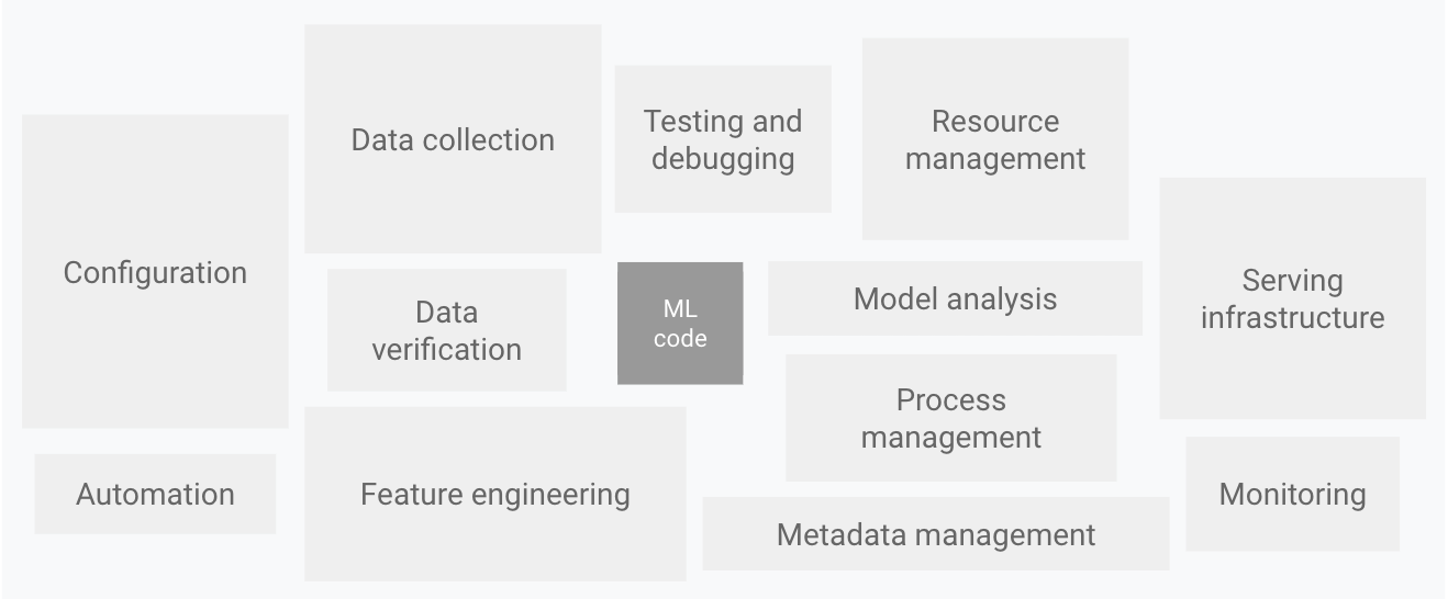 Components of an ML system
Diagram by Google
Components of an ML system
Diagram by Google
Anecdotally, think about the last time you trained a decent ML model in a Jupyter notebook, only to realise that productionising it would take even longer than the initial experiment/model training itself? All those ‘one-off’ loads of data, ‘one-off’ preprocessing and feature engineering and filters on querying source data suddenly now becomes a huge task to productionise. Not to mention all the infrastructure needed for logging, serving the model and measuring performance speed etc.
Therefore, understanding the various layers and architectures of machine learning system is a key part to building a successful ML system.
Main types of ML system architectures
There are broadly three main types of ML system architectures.
| 'Online' Pattern | 'Offline' Pattern | 'Streaming' Pattern | |
|---|---|---|---|
| Training | Batch | Batch | Streaming |
| Prediction | On-the-fly or 'live' | Batch or 'offline' | Streaming |
| Serving mechanism | Via REST API | Via SQL database | Via Streaming queue |
| Prediction speed | Medium | High | Low |
| Ease of implementation and management | Medium | Easy | Hard |
Each one has its pros and cons. For example, an ‘offline’ model is generally more ‘static’ as its only re-trained every once in a while. However, in contrast, ‘online’ models are generally ‘dynamic’ and can adapt to real-world conditions quicker (e.g. a new product is released).
There are some quirks for time series forecasting, as the model must be retrained on every single time series that it gets. You can’t have a model that forecasts the sales of customer A be used on customer B.
Google’s advice: use a static model if the data doesn’t really change, but you need to still monitor your input data for change. Like the sea level, even things that you think don’t change actually still do over time.
My personal approach: start with an ‘offline’ pattern, which is easier to implement and get up and running, then scale it up to an online pattern if needed.
Components of an ML system
Conceptually an ML system can be thought of as 4 layers, with each layer’s output being the input of the below layer:
-
Data Layer - gathers all the required data from various sources and preprocessing them into standardised formats.
-
Feature layer - generating feature data in a transparent, scalable and extensible way.
-
Scoring Layer - houses the models which transforms features into predictions. The model is trained in this layer.
-
Evaluation Layer - evaluates how the well model performs with its prior version (i.e. delta testing), as well as how well the model performs between training vs real data. This layer is also responsible for monitoring all the other layers to see whether they are performing correctly.
Each layer is essentially like a stage in a data workflow. Separating your system into these four layers makes it much easier to extend and maintain your system. For example, if the data source changes (say from a SQL server database to a PostgreSQL database) you just need to update the data layer.
Ensembled Learning - multiple models operating in harmony
Like the old adage goes - if you can make one you can make many. Likewise, at its core, a machine learning model essentially:
Input -> Do Something -> Output (usually a prediction)
So you can further extend this chain to:
- The output of one model goes into another model
- The output of many models goes into another model
You likely may have noticed that option 1 is essentially how hybrid systems work - the output of a rules-based model is fed into the machine learning model. But when you have many machine learning model outputs fed into another model, this is known as ensembled learning.
Bagging vs Boosting
Broadly speaking there are two ways to ‘ensemble’:
- Boosting - each model is trained emphasising on the prior model’s ‘mistakes’ to improve the overall model. That is, the model is basically learning from the prior model’s mistakes.
The best example of boosting is Extreme Gradient Boost decision trees. In each iteration (i.e. epoch), the tree learns from the prior version’s mistakes and incrementally improves itself. The final prediction is whatever the final model, which has learnt from all the mistakes from its predecessors, predicts.
- Bagging/Bootstrapping - each model ‘votes’ on a prediction and the majority vote is selected as the prediction. Each model is given a random subset of the training data (both features and data points) to ensure they don’t end up being the same model repeated multiple times.
The best example of bagging is the Random Forest algorithm - you create, say 100 decision trees which classify whether a picture is a dog or cat. If 60% of trees predict cat, then the final prediction is cat.
Best Practices when using Ensembled Learning
When determining inputs for one model to another, you should pick one of the following, but never both:
- Parts factory approach - you only take the inputs into the prior model
- Assembly plant approach - you only take the output from the prior model
If you use both approaches you’ll end up getting compounding errors. That is, incorrect inputs into the prior model will result in incorrect output from the prior model, so you get double the amount of incorrect stuff coming in.
Practical Example - Energy Forecasting
Below is a high-level example of an machine learning model with multiple components from one of my previous work projects.
As you can see, to get to the final model, there are multiple intermediate steps and other models in between. However, in the final model (Energy Saving Model), it only takes the output from the prior model and does not take the input of the prior model.
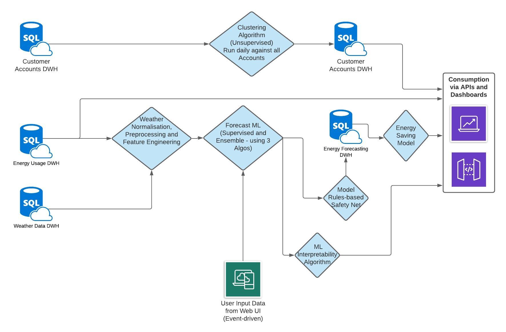 Example of machine learning system with multiple models
Delta Testing - the regression test for ML systems
What makes ML systems complex is not just the code changing, but the input data may change that results in new algorithms developed by the model during training. Therefore, if you want to test just code changes, you need a way to exclude the effects of data changing.
In software engineering, regression testing is a suite of unit tests, integration tests and other types of tests to ensure that a new feature or iteration does not cause the system to ‘go backwards’. That is, the overall functionality has not regressed. The idea is to pick up on difficult to detect errors or bugs that only pop up when all the components are online.
In machine learning, the concept of regression testing is generally in the form of delta testing - that is, the current system does not have an overall predictive performance worse than the prior version.
An example is incorporating a Pytest test which covers this - testing the F1-score for the current classification model vs the prior version:
def test_model_prediction_delta(self, previous_file='test_predictions.csv'):
  '''
  GIVEN the current model
  WHEN I get the prior model's results and training data
  THEN I can compare the performance of prior vs current models
  '''

  # Load prior model results which has training dataset
  prior_model_df = pd.read_csv(previous_file)
  prior_model_predictions = prior_model_df.prediction.values
  train_df = prior_model_df.drop(columns='predictions')

  # Predict Current Model
  current_df = model_predict(train_df)
  current_model_predictions = current_df.prediction.values

  # Calculate accuracy and differences
  current_results = evaluate_metrics(current_model_predictions, metric='f1', method='average')
  prior_results = evaluate_metrics(prior_model_predictions,  metric='f1', method='average')

  # Assertion
  assert current_results > prior_results
A few things to keep in mind if you use tests like this:
-
The European Union General Data Protection Regulations (GDPR) may restrict your ability to reproduce a training dataset, as it may constitute storing personal data outside of approved location
-
Make sure your training data to evaluate the current and prior model is the same - snapshot the data! Also remember to pass in the data in the same order, e.g. using a ORDER BY in a SELECT statement. Otherwise, you may end up getting different results every run.
Closing Thoughts
It’s amazing how much a machine learning system can make or break on its non-ML components. Good feature engineering, incorporating great heuristics and having scalable/transparent workflows are key ingredients to good machine learning.
Counter-intuitively, despite the focus of ML on algorithms, spending more time on the components besides the algorithms may yield the greatest results.