Data Science/Analytics Pitfalls
So following on my prior blog post on common data science/analytics pitfalls, we’ll now focus on pitfalls more specific to machine learning!
Note that while focused on ML, these pitfalls are equally applicable statistical/data science work in general.
Heads up: this blog post is intended to be used as a ‘mini-wikipedia’ for future references (hence the length). Feel free to skip use the table of contents to skip to the section that interests you.
- Data Science/Analytics Pitfalls
- Not formulating your question correctly
- Golden Hammer Bias
- Not evaluating your model properly
- Not using or developing a baseline model
- Not doing proper out-sample testing
- Not having a failsafe or automated validation layer for ML/AI
- Using machine learning for non-stationary environments
- Using biased datasets/processes to train machine learning models
- Closing Thoughts
Not formulating your question correctly
Data science/analytics is about addressing real-world business problems - it’s easy to get caught up in all the data and magic.
Determine which type of data work this is
Before you begin any form of data work, you need to determine which type of outcome you are trying to achieve. IBM has identified 5 types of analytics:
- Planning Analytics - What is our plan?
- Descriptive Analytics - What happened?
- Diagnostic Analytics - Why did it happen?
- Predictive Analytics - What will happen next?
- Prescriptive Analytics - What should be done about it?
Descriptive analytics involves insight into the past, analysing historical data. It is more about what has happened and not used to draw inferences/predictions. IBM considers descriptive analytics to encompass 5 stages:
-
Determining your business metrics/KPIs - e.g. improving operational efficiency or increasing revenue
-
Identify and catalogue the data required - whether from databases, reports, spreadsheets, etc.
-
Collect and prepare the data - cleaning, transformation, etc.
-
Analyse the data - including summary statistics, clustering etc.
-
Visualise/present the data - charts and graphs to visualise the findings
 Who, what, when, where, why?
Photo by Gerd Altmann from Pixabay
Who, what, when, where, why?
Photo by Gerd Altmann from Pixabay
Diagnostic Analytics further extends descriptive analytics, assessing the descriptive datasets and drilling down/isolating the root-cause of an issue.
Predictive Analytics, on the other hand, is focusing on predictive modelling/forecasting. It is about predicting possible future events and their probability.
Examples of predictive analytics include:
- Forecasting future demand to improve supply chain
- Risk and detect fraud
- Forecasting future growth areas to focus marketing and sales strategies
Prescriptive Analytics, finally, builds upon descriptive, diagnostic and predictive analytics to identify the best course of action. It involves analysing the predicted outcomes and determining the impact of those outcomes.
For example, in the energy industry:
-
Descriptive analytics shows the last 5 years have shown a 300% increase in electricity demand. This has strained the existing electrical grid capacity to 90%.
-
Predictive analytics using machine learning forecasts demand will jump by another 200% in the next 2 years.
-
Prescriptive analytics can identify which particular assets/infrastructure need to be upgraded to meet this forecasted demand.
Knowing which type of analytics you are trying to achieve will frame many questions and starting points, including your hypothesis (as stated below).
Your hypothesis is your starting point
The concept of a hypothesis always start with formulating two things:
- What is the default position if the question isn’t answered (i.e. the null hypothesis)
- What is the alternative position if the question is answered (i.e. the alternative position)
 Hypothesis are important for experiments!
Photo by PublicDomainPictures from Pixabay
Hypothesis are important for experiments!
Photo by PublicDomainPictures from Pixabay
So you can see two scenarios in which the data question is very different:
Scenario A
- Default Position - we don’t sell cupcakes
- Alternative Position - we sell cupcakes if it is profitable
Scenario B
- Default Position - we keep selling cupcakes
- Alternative Position - we stop selling cupcakes if it is not profitable
You can see how you frame the question will totally change how you approach the data question. Proving selling cupcakes is profitable is a different exercise to showing selling cupcakes is not profitable (e.g. if you don’t sell any cupcakes, does that count as profitable?)
Another example is if your framed a question like this: everyone is guilty until proven innocent. Even if you come up with the best data science model, people are going to wonder how on earth did you even come up with such a crazy question to begin with!
Golden Hammer Bias
The ‘golden hammer’ is a cognitive bias where a person excessively favours a specific tool/process to perform many different functions.
A famous quote attached to this theory summarises it nicely:
If the only tool you have is a hammer, every problem you encounter is going to look like a nail
The golden hammer bias can lead to a ‘one-size-fits-all’ model or approach to a data issue. In statistics/ML this is also known as the ‘No Free Lunch Theorem’. That is, there isn’t’t a single algorithm that is best suited for all possible scenarios and data sets.
Not evaluating your model properly
Every data science model needs to have a method to measure how well it is doing. The way to measure this is via evaluation metrics. The common types of evaluation metrics include:
Regression Problems - predicting an actual value (e.g. tomorrow’s weather)
-
Mean Absolute Error (MAE) and Root Mean Squared Error (RMSE) - essentially measures the average error of the model. It is a measurement of error, so the lower the better. Due to its calculation, RMSE penalises bigger errors more than MAE.
-
Mean Absolute Percentage Error (MAPE) - Average % error of the model (lower the better). However neither RMSE, MAE, MAPE show the direction of errors (over or under).
-
Adjusted R-squared score - essentially measures the correlation between the predicted values and the actual values. It is a measurement of goodness of fit, so the higher the better.
-
Akaike Information Criterion (AIC) - essentially measures how well the model performed, factoring in how complicated the model is. The lower the AIC, the more generalised it is and better the model (i.e. less likely overfitted). This metric is mainly used for time series forecasting, where there isn’t enough training data to compare which model performed better.
For every classification problem, expressed using a confusion matrix, you can see what the possible outcomes are:
| Actually has Cancer | Actually does not have Cancer | |
|---|---|---|
| Predicted Has Cancer | True Positive | False Positive |
| Predicted does not have Cancer | False Negative | True Negative |
Using the above matrix, you can see there’s multiple ways to evaluate the classification problem:
- Accuracy - how many correct outcomes the model predicted
- Precision - essentially measuring rate of true positives and false positives
- Recall/Sensitivity (i.e. True Positive Rate) - essentially measuring rate of true positives
- Specificity (i.e. Inverted False Positive Rate)- essentially measuring rate of true negatives and false positives
- Balanced Accuracy (i.e. F1 score) - combination of the above.
The relationship between them all is defined as:
Accuracy = (True Positive + True Negative) /
(True Positive + False Positive + False Negative + True Negative)
Precision = True Positive / (True Positive / False Positive)
Recall/Sensitivity = True Positive / (True Positive + False Negative)
Specificity = True Negative / (True Negative + False Positive)
False Positive Rate = (1 - Specificity)
F1 score = 2 / ((1 / Precision) + (1 / Recall))
 Know your target!
Photo by 3D Animation Production Company from Pixabay
Know your target!
Photo by 3D Animation Production Company from Pixabay
When to pick what evaluation metric
Which evaluation metric is selected affects what you are achieving. A common type of classifcation will involve an ‘imbalance’ between the number of positives vs negatives. For example, 99.999% of the population will not have a particular cancer and only 0.001% does.
When you have an imbalanced problem, using accuracy as an evaluation metric wouldn’t be suitable. That’s because if I needed to predict whether a person has cancer, using the above scenario, I could say ‘no cancer’ and be right 99.999% of the time.
Therefore, in these instances, you can’t use accuracy as a measurement. You wouldn’t want your predictive model to do too many false negatives and false positives, but you may consider false negatives to be much more worse. That is, someone that had cancer but the model said they didn’t.
In these instances, an appropriate method would be using Recall, which factors in how many false negatives the model has.
- Use Precision if you care more about true and false positives - e.g. spam emails
- Use Recall if you care more about false negatives than false positives - e.g. cancer prediction
- Use Specificity if you care more about false negatives - e.g. predicting violent crimes
- Use F1 Score if you have an imbalanced dataset
- Use AUC-ROC score if you have a more balanced dataset (explained below)
It is sometimes a trade-off (illustrated by the AUC-ROC curve)
In an imperfect world, true vs false positive/negative will be a trade-off:
- If you predict no one has cancer, you get 0% false positives but 100% false negatives
- If you predict everything has cancer, you get 100% false positives but 0% false negatives
Some algorithms allow you to tweak the probability threshold/cut-off in which you consider something is true or not.
For example, if you took a 50% threshold (default position) - red indicates false negative and orange indicates false positive:
50% Probability Threshold
| Patient | Probability of Cancer | Model's Prediction (applying 50% threshold) | Actually has cancer |
|---|---|---|---|
| 784 | 10% | N | N |
| 123 | 30% | N | Y |
| 585 | 40% | N | N |
| 1156 | 50% | Y | Y |
| 9725 | 55% | Y | N |
| 29823 | 90% | Y | Y |
For example, given the consequences of a false negative is much higher than false positive, you might set the threshold to be 30% (rather than 50%). This will reduce number of false negatives, but it will increase number of false positives:
30% Probability Threshold
| Patient | Probability of Cancer | Model's Prediction | Actually has cancer |
|---|---|---|---|
| 784 | 10% | N | N |
| 123 | 30% | Y | Y |
| 585 | 40% | Y | N |
| 1156 | 50% | Y | Y |
| 9725 | 55% | Y | N |
| 29823 | 90% | Y | Y |
If you then took a more extreme approach and set the threshold to 10%, you would get basically no false negatives, but a lot of false positives:
| Patient | Probability of Cancer | Model's Prediction (applying 10% threshold) | Actually has cancer |
|---|---|---|---|
| 784 | 10% | Y | N |
| 123 | 30% | Y | Y |
| 585 | 40% | Y | N |
| 1156 | 50% | Y | Y |
| 9725 | 55% | Y | N |
| 29823 | 90% | Y | Y |
The curve that illustrates the false and true positive rates at various probability thresholds is known as the Receiving Operating Curve (ROC):
ROC Curve = False Positive Rate (X axis) vs. True Positive Rate (Y axis)
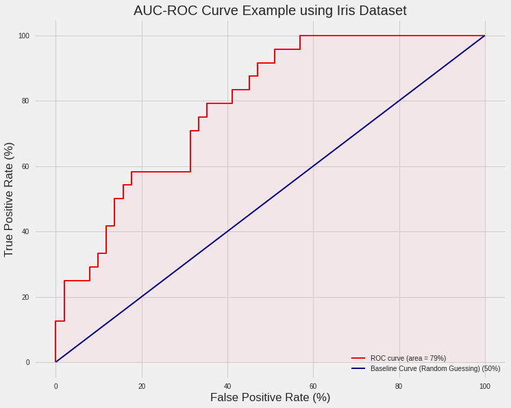 AUC-ROC Curve Example
We then calculate the Area Under this Curve to get a percentage. The baseline is 50%, which is random guessing and assuming you would get 50% wrong 50% right. Therefore, any model with a AUC-ROC score less than 50% is considered not good (as random guessing would fare better).
Knowing what you are measuring and what your ultimate goals are is a crucial important in building a good model!
Percentage of error is not always appropriate
Another example is not using Mean Absolute Percentage Error (MAPE) properly. Because in forecasting you could end up being way off, sometimes it’s not appropriate to use a percentage. Therefore, your model could be 1,000,000% inaccurate!
Furthermore, over forecasts are more heavily ‘penalised’, as the maximum amount of error for an under forecast is 100%. To illustrate, we’ll do a simple calculation:
- Actual value is $1,000
- Forecast value is $1,200
- Therefore your % error = ABS($1,200 - $1,000)/$1,000 = 20%
Now take the same scenario, but with more extreme numbers:
- Actual value is $1,000
- Forecast value is $120,000
- Therefore your % error = ABS($120,000 - $1,000)/$1,000 = 119,000%!
But if you under forecasted by a lot, there’s a cap on the error:
- Actual value is $1,000
- Forecast value is $3
- Therefore your % error = ABS($3 - $1,000)/$1,000 = 99.7%! (Your number can never go above 100%)
Furthermore, if your actual value is $0, then you obviously can’t divide by error so you can’t even calculate a MAPE!
So picking the right evaluation metric is important as if you can’t reliably measure how well your model is doing, you can’t improve it (or prove it actually works).
Not using or developing a baseline model
A common mistake for people who are starting out in data science is jumping straight into the problem, building a machine learning model and calling it a day!
Ultimately the model needs to provide value-add, either in more accurate predictions, time saved, capability increased etc. To do this, however, you need to have a baseline.
A baseline model is a model that does a prediction using naive/simple techniques. It is analogous to comparing your model to a random person guessing. It is important to note that you should not use a baseline as a final model. It is merely to illustrate/prove that your model can at least beat a baseline.
It is surprisingly hard to beat a decent baseline model - for example, in forecasting, naive forecast methods often beat many types of machine learning models. You can see an example in my previous blog post on electricity forecasting.
Baselines are also important when there are imbalanced datasets - such as banking fraud prediction models. If 99.9% of transactions are not fraudulent, blind guessing ‘not fraudulent’ for every single transaction will yield a 99.9% accuracy. So therefore, your prediction model should at least beat this.
 A steady baseline
Photo by Thanks for your Like • donations welcome from Pixabay
A steady baseline
Photo by Thanks for your Like • donations welcome from Pixabay
Naive Baseline Models
These are called ‘naive’ because they apply a very simple rule to predict a value.
For regression problems, these include:
-
Persistence model (for time series forecasting) - e.g. one-year persistence model means taking 1 August 2019’s value to predict 1 August 2020’s value
-
Zero Rule Algorithm using mean, median or most frequent value - i.e. predicting the future value using the mean/median or most frequent value in the existing dataset. They are known as ‘Zero Rule’ due to their simplicity and only predicting the same value for all scenarios (i.e. no rules).
For classification problems, these include:
-
Zero Rule Algorithm using median or most frequent value - i.e. predicting the future value using the median or most frequent value in the existing dataset
-
Dummy Estimator using stratified predictions - i.e. it makes a guess based on how frequent an a category appears. For example, in a dataset, 30% of the customers are ‘low risk’, so therefore it will guess ‘low risk’ 30% of the time.
-
One Rule Classifier - you select the feature that is the best estimator for the target and use that as the ‘rule’. For example, if you have a dataset for customer sales, ‘one-rules’ to predict whether a customer buys a produce could be:
- If Premium_Customer_YN = ‘Y’ -> Predict ‘Y’
- If Premium_Customer_YN = ‘N’ -> Predict ‘N’
Simple Model as a baseline
For the purposes of doing a baseline, there’s a few algorithms that provide a good starting point to improve on.
The purpose of using these models isn’t to get a final model, but rather have something to compare to and demonstrate that any further ML work has more value-add. These include:
-
Logistic Regression model - like linear regression, logistic regression can be ‘universally’ applied to a classification problem to get a decent baseline model. Furthermore, logistic regression allows you to tweak the probability threshold - e.g. if you get the threshold at 80% for predicting fraud (Yes vs No), then the model will only say ‘Yes’ if there’s at least a 80% probability there’s fraud. This allows you to effectively have a dummy estimator if you get the threshold to 0% or 100%. For regression problems, common types of baseline models include:
-
ElasticNet linear regression model (L1 + L2 Regularization) - linear regression is conventionally considered a baseline model, because of how ‘universal’ it can be applied to a regression problem. For the purposes of baselining, you won’t need to consider the linear regression assumptions, as you won’t end up relying on this for your final model.
Importantly, keep the features simple. Simple features means creates a simple model, resulting in a baseline model and metrics that can be used to evaluate your subsequent more complex models.
Rules-based baseline models
Another form of baseline is a rules-based approach (a.k.a. heuristics-based modelling) that reflects the current business processes.
Many of these rules may be derived from years of business experience and known practices already adopted. This makes sense, given the goal of a machine learning model is to improve existing processes.
I discuss more about hybrids and heuristics in another blog post.
The end result may be that a hybrid model with 70% rules-based and 30% machine learning will outperform a 100% machine learning model. After all, the focus is on a model that performs the best, not uses the fanciest technology/algorithm.
Not doing proper out-sample testing
In general, when you develop a model (whether machine learning or rules-based), you need to split the data between a training dataset and evaluation/testing dataset. The idea is your machine learning model should never see the evaluation/testing dataset when it’s training.
A simple split method is randomly selecting 70% of the data for training and 30% for testing. The reason you pick a random sample is to avoid data skewers (e.g. picking all the customers from a certain address).
More comprehensive methods such as K-fold cross validation can be used to further improve this splitting - it sub-divides the dataset K times (e.g. 10 times) and for every sub-division, it will further do a train-test split.
Scikit-Learn has a great visualisation of how this works:
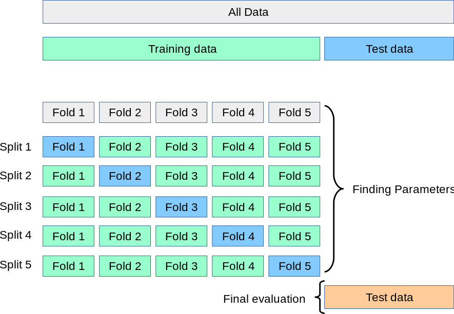 K-fold Cross Validation.
Diagram from Scikit-Learn
K-fold Cross Validation.
Diagram from Scikit-Learn
Out-sample testing is when you test your model using data that you didn’t use to train your model. You do this to prove that your model ‘truly’ can predict stuff it has never seen before. It is analoguous to exams for humans - you do your study and now you need to prove you can do it with something you’ve never seen before.
There are a few do nots:
-
Don’t abuse out-of-sample data by building a model, testing it on the out-of-sample data and constantly going back and forth. What you end up with is basically treating the out-of-sample data like your training data.
-
Avoid getting ‘inspiration’ or ‘trends’ from your out-of-sample dataset and then testing it on the same dataset. If you have a ‘trend’ you want to test it, do it on a dataset that you’ve never seen before.
-
Out-sample data is not representative of the real world and has skewers/biases in it
-
Your out-sample data isn’t really out-of-sample and is part of your training dataset
If you can’t reliably test how well your model performs with out of sample data, you can’t figure out how well it really performs!!
Not factoring in the Bias-Variance Trade-off
When you create a machine learning model, there are two competing things that constantly battle it out:
- You want your model as simple as possible
- You want your model to cover as many scenarios as possible
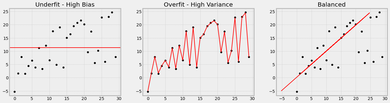
If your model does number 1 very well, it is biased and underfitting, because it ignores a lot of the dataset’s characteristics.
If your model does number 2 very well, it has high variance and overfitting, as it is trying to cover every single scenario possible.
You can’t have it both ways!
When training a model, there will be a point when the model will stop generalizing and start learning the noise in the dataset. The more noise it learns, the less generalised it is and the more horrible it is at making predictions on unseen data.
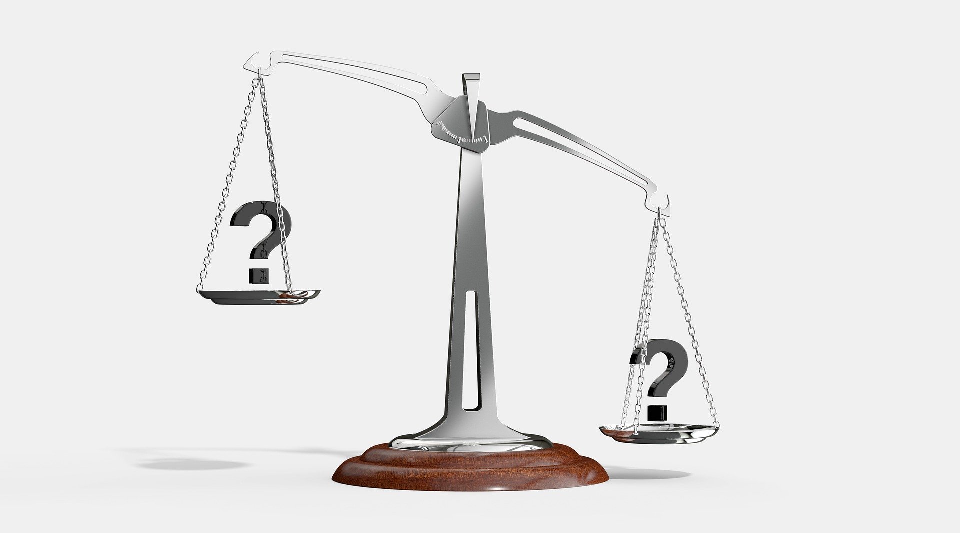 Getting the balance right
Photo by Arek Socha from Pixabay
Getting the balance right
Photo by Arek Socha from Pixabay
An example of a model underfitting is a model classifying dog vs wolves. The algorithm was given images of dogs and wolves to train on. However, the training images always had dogs in grass and wolves in snow. Therefore, rather then learn the general features of dogs vs wolves, it classified anything in snow a wolf and anything in grass a dog!
However, on the other end of the spectrum, being too specific can be problematic - a common analogy is a student that studies for an exam. The student can:
- Study the material and do the practice exam questions
- Remember all the practice exam questions and answers off by heart
Now if the student did the exam and 100% of the questions were the practice exam questions, then scenario 2 would mean they score 100%! But the real world doesn’t work like that, so you would expect Scenario 1 to give better outcomes because they are more ‘generalising’ their knowledge to cover more scenarios.
There is a constant trade-off between Bias-Variance - the more it goes one way, the less it’ll go the other way. On the one hand you want your machine learning model to be able to perform very well predicting the training data (i.e. the ‘practice’ exam), but at the same time if the model performs 100% it means overfitting (i.e. they are only good at answering the practice exam, not questions in general).
 Aim for the Goldilocks!
Overfitting is much more common than underfitting, as when you train a model, you’re always trying to get the possible metric! You keep going, tweaking until you get 90%, 95% and then 100% accuracy. Wait hold on - that’s a sign of overfitting!
You then run the model on out-sample data and its doing 30% accuracy.
A great example and parody of overfitting by XKCD:
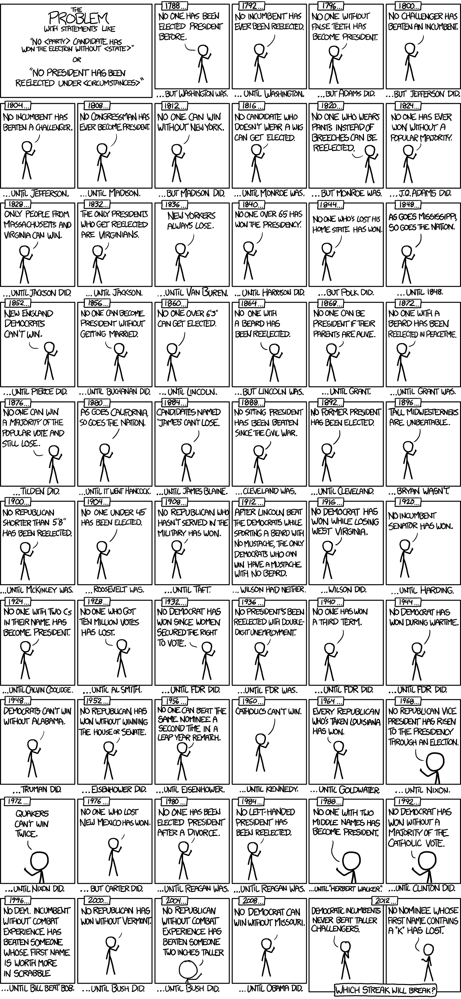 Image from XKCD, used under a Creative Commons Attribution-NonCommercial 2.5 License.
Not using percentages correctly
Percentages are a great way of describing data - it is a type of reference that many people are comfortable with. Saying 10% of sales or 50% of people is easy to understand.
However, because percentages are not absolute numbers, there’s potential for manipulation and confusion.
I’ve noted some tips below.
Don’t use percentages when the values can be negative
When values can be negative, it means percentages won’t make sense. For example, you are measuring the increases/decreases of the robberies in a city for a particular year:
| Suburb | Increase/Decrease to # of Robberies |
|---|---|
| Suburb A | +3,000 |
| Suburb B | -2,000 |
| Suburb C | +5,000 |
| Suburb D | -4,000 |
| Suburb E | +3,500 |
| Total Net Increase | 5,500 |
Taking the above, you can calculate that Suburb A contributed to 3,000 out of the 5,500 net increase to robberies and therefore 54.5% of the robbery increases came from Suburb A!
But that’s very misleading, because if you take the same logic to the other suburbs:
- Suburb A contributed 54.5%
- Suburb C contributed 90.9%
- Suburb E contributed 63.6%
Not a very useful metric!
Don’t use percentages when the total of the values can be over 100%
For example, the famous Colgate Ad which said 4 out of 5 of dentists recommend Colgate was deemed to be misleading by the UK Advertising Standards Authority.
What actually happened was dentists were asked which toothpastes to recommend. 80% (or 4 out of 5) dentists provided a list and Colgate was in 80% of lists. However, the list may look like:
- Colgate
- Oral B
- Sensodyne
Therefore, by Colgate’s definition, you could get something absurd like: 80% of dentists recommend Colgate, 100% recommend Oral B and 70% recommend Sensodyne. Gives a totally different (and somewhat confusing) meaning!
Another way to think of it is: if I can’t visualise it in a pie chart, then it doesn’t make sense to use percentages.
 I don’t think you can plot 1000% on a pie chart…
Photo by Clint Post from Pixabay
I don’t think you can plot 1000% on a pie chart…
Photo by Clint Post from Pixabay
Comparing percentages with different bases
When you represent trends and growths in percentages, it helps illustrate the point, but sometimes is misleading. After all, 80% of $10 is very different to 80% of $1 million.
An example is if the chance of cancer from taking a drug was 0.00010%. If you then take a new vesrion of the drug, your chances could go up to 0.00018%. Technically speaking that is an 80% increase, but saying the drug increases your chance of getting cancer by 80% seems misleading. After all, the actual number is still very small.
A less misleading way would be saying something like: your chances of getting cancer go from 0.00010% up to 0.00018%, a total increase of 0.008%.
XKCD sums it up greatly:
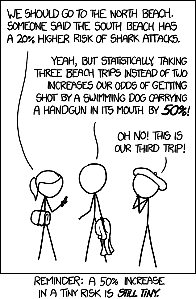 Image from XKCD, used under a Creative Commons Attribution-NonCommercial 2.5 License.
Data leakage - the model is cheating
A key principle is preparing the data for machine learning, you split the data into at least two parts (or more if you do cross validation):
- a training dataset which contains the ‘questions’ (features) and the ‘answers’ (target)
- a test dataset which should stimulate real world, yet-to-be-seen data. The model should never see the ‘answers’ (i.e. target) in this dataset.
Data leakage is when the training data for a machine learning model contains information which wouldn’t be available in a real prediction scenario. That is the model is ‘cheating’ and will result in a very good performing model during training, but not so good (or even rubbish models) during actual production.
Models are usually designed to predict the future, but are trained using historical data. Therefore, you need to be careful on what data the model should have available at the point of its decision/prediction.This includes when you preprocess data (e.g. imputers or scalers) - if you do it on the whole dataset before doing the train-test split, your model has had a sneak peak of the attributes of the test dataset!
If data that shouldn’t exist at the point in time of prediction exists in the dataset and you use it for training, your results will be distorted. For example, if you want to predict the gold price for the next 5 days:
| Date | Gold Price |
|---|---|
| 2021-08-02 | ? |
| 2021-08-03 | ? |
| 2021-08-04 | ? |
| 2021-08-05 | ? |
| 2021-08-06 | ? |
The model at any point of prediction can only know what the gold price is up to that point. That is, when you train the data, you cannot do this:
| Date | Gold Price |
|---|---|
| 2019-08-02 | 1718.8 |
| 2019-08-03 | 1700.1 |
| 2019-08-04 | 1710.5 |
| 2019-08-05 | 1735.1 |
| 2019-08-06 | ? |
Then do this:
| Date | Gold Price |
|---|---|
| 2019-08-03 | 1700.1 |
| 2019-08-04 | 1710.5 |
| 2019-08-05 | 1735.1 |
| 2019-08-06 | 1720.9 |
| 2019-08-07 | ? |
The model at the point of predicting the next 5 days won’t know what the next 4 days of data is. Therefore, you are effectively training the model on future data (fortune telling to the extreme)!
Another example is data that is updated after the fact. For example, you are building an algorithm trying to predict defaults for customer loans. Your dataset comes from the company’s CRM which has a credit score field. However, you later realise that this when customer defaults, the CRM will update their credit score to be 0.
You then have to exclude this feature in your algorithm - otherwise model will say 100% correlation that 0 score = default. Which is true, but the 0 score was only updated after the customer defaulted.
Another good example is a model designed to predict whether a patient has pnuemonia - the dataset has a feature ‘took_antibiotic_medicine’, which is changed after the fact (i.e. you take the antibiotics after you get pneumonia).
Therefore, using this to predict whether someone has pneumonia is a lousy model - in real life, a patient doesn’t get antibiotics until they are diagnosed with pneumonia.
 Not a crystal ball!
Photo by Uki_71 from Pixabay
Not a crystal ball!
Photo by Uki_71 from Pixabay
To avoid this, you should try to:
-
Have some hold-out datasets - this is data that is completely not used in the entire ML process and only used at the very end to evaluate the model
-
Always do train-test split before you do preprocessing
-
Have a cut-off date - this is very useful for time series data. You specify a date where all data after a particular point is ignored.
-
Ensure duplicates don’t exist - this will avoid the same data be in both the training and test datasets
Not having a failsafe or automated validation layer for ML/AI
Occasionally, machine learning models will generate some crazy results that are totally unexpected. It may be the result of incorrect data (e.g. someone actually wrote 170km for their height instead of 170cm). If these aren’t picked up in the preprocessing, it could end up with some obscure outcomes.
Unlike humans, ML models don’t ‘self-correct’ and therefore it’s important for humans to build in a separate layer of automated validation or ‘failsafe’. The idea is this layer checks the output to the model and applies some baseline checks to ensure the outcome is not completely unexpected.
This layer is generally rules-based and reflects the fundamental ‘red lines’ of the organisation/business. For example, having a baseline safety check so a system will never grant a home loan for $1.
Having this separate layer is important as you can’t account for everything in the ML model. A ML model won’t know what your fundamental red lines are, but you as a human do.
As the old saying goes, “you can plan to fail, but you shouldn’t fail to plan.”
Using machine learning for non-stationary environments
Stationary means the underlying rules relating to the data haven’t changed. So therefore if the rules changed, your it is non-stationary.
If it’s very obvious past doesn’t indicate future, then you can’t use the past to predict the future. It’s like trying to predict how many people will drive tomorrow using data from 200 years ago (when they didn’t have cars).
This error is quite easy to make - say for example, you need to make a churn model that predicts whether a customer calling in will likely to leave your company. If you only have data for March available and March has a frenzy sale, you can’t really use that to predict April churn/sales. Why? Because the underlying rules relating to the sales changed (there’s no more frenzy sales)!
Furthermore, factors such as new customers, new products, seasonality etc. all come in. This is why the older the historical data is the less likely it can be used for predictive modelling - there’s just too much that could’ve changed.
Nowadays deep learning algorithms and more advanced reinforcement learning techniques can potentially overcome this via the algorithm ‘learning’ the changes. However, it is important to still keep this in mind - otherwise you will see big drops in your model’s performance.
Using biased datasets/processes to train machine learning models
At its core, machine learning models learn from existing real world data and all the above conventional knowledge on data science/analytics is your data, processes and model should reflect the real world.
However, this is very problematic if your data reflects historical biases, discrimination and other unfair events. By extension, you can see that this will result in training biased AI/ML, which has become more and more in the spotlight recently.
The European Union’s General Data Protection Regulation (Rectical 71) actually makes it unlawful for a person to be subject to a decision based on a discriminatory automated process!
A famous example of this was a machine learning model that Amazon created for recruiting staff. After a while, they realised that the machine learning model was biased against women, because historically, recruitment favoured men over women.
Therefore the model, using this historical data, ended up favouring men applicants over women too. The historical discrimination and bias was further entrenched!
 Just because I’m red doesn’t mean I’m less important!
Photo by Ronile from Pixabay
Just because I’m red doesn’t mean I’m less important!
Photo by Ronile from Pixabay
Other high-profile examples of discriminatory AI and models include:
-
Correctional Offender Management Profiling for Alternative Sanctions (COMPAS) - an algorithm designed to predict whether a criminal defendant would likely reoffend, was used by US courts, correctional facilities, etc. as a factor in their decision-making. Unfortunately, historically bias against black defendants in the criminal justice system was entrenched and the algorithm was arguably biased against black defendants.
-
Google Photos categorisation algorithm - the algorithm categorised images in Google Photos, such as ‘dog’, ‘car’, etc. It was discovered there was a significant lack of photos of dark-skinned people fed to train the algorithm and therefore it erroneously labelled some dark-skinned people as ‘gorillas’. Oh dear!
Unfortunately to address this issue is almost to contradict all the above points I mentioned, as essentially your model has to deliberately not reflect the historical reality to not be biased. So in a way, if you were to apply your model against historical data, it should in theory be inaccurate, because it doesn’t result in biased results like the historical actual data has.
Google AI has outlined some Responsible AI Practices. I’ve summarised a few high-level tips:
-
Ensure you use enough test data that is inclusive/fair - for example, including a significant enough portion of cultural, racial, gender, religious diversity
-
Ensure you use test data that reflects the future real world use - for example, if you are going to deploy a speech recognition algorithm globally, test it on people with different accents
-
Have people play ‘devil’s advocate’ and adversarially test the system with edge cases to see how well it performs
As we become more and more reliant on automation and AI/ML, the effect of bias in these models becomes a bigger issue.
Closing Thoughts
So this wraps up my 2-part blog on common data science/analytics pitfalls.
Hope you learnt something new!