Kimball Dimension Modelling - what is it?
Many data lakes and warehouses are architectured with two main data models:
- Kimball Dimension Modelling
- Data Vault Modelling
Kimball Dimension Modelling is considered the more popular one and sometimes known as the ‘bible’ of data warehousing. For most use cases, it fits surprisingly well and the best part is it is easy to explain to non-technical laypersons.
The value of being able to explain a large data warehouse that encompasses an entire organisation in simple terms to business stakeholders is a very important feature!
This blog article will discuss these rules in a more simpler approach using examples, as well expand on each point with other parts of Kimball.
Kimball 101
Kimball dimension modelling has a strong focus on identifying the business processes - the idea is your model should reflect the real world, not the other way round.
Each table that is built into the data warehouse falls into two types:
-
Dimensions - these are tables that describe attributes in the real world - e.g. customer name, address, phone number
-
Facts - these are data points that will be measured and usually ultimately feed into some form of Key Performance Indicator (KPI) or metric - e.g. sales by region, customer growth by site
Dimensions should ultimately reflect real world business processes - for example, for every stage in a supply chain. Furthermore, every fact table should ultimately have a linkage to a dimension - after all, what’s the point of measuring something if it’s not related to a real world business process.
Kimball dimension modelling involves 4-steps:
- Choose the business process
- Declare the level of detail (ie. grain)
- Identify the dimensions
- Identify the facts
In Kimball terms, the level of detail is known as the grain. Determining the grain is an important detail - for example, do you record your sales amounts by store, city, region or country?
The Snowflake and Star Schema
The dimension and fact tables form a web of interconnected datasets in the data warehouse. There are two main types of connections - Snowflake and Star.
We’ll focus on Star schema for simplicity purposes.
The star schema is a design method that has multiple fact tables that join up multiple dimension tables. The main ‘stars’ (excuse the pun) of the design are the fact tables.
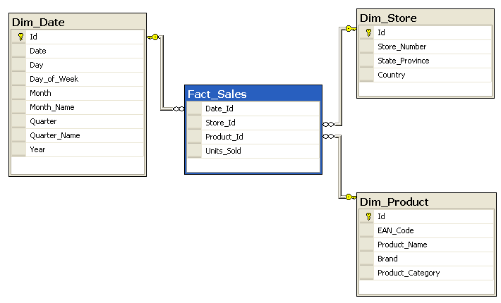 Example of a Star Schema
Image By SqlPac at English Wikipedia, CC BY-SA 3.0, Link
Example of a Star Schema
Image By SqlPac at English Wikipedia, CC BY-SA 3.0, Link
To complete this design, every fact table must have a linkage to the dimension table via ‘keys’. Usually these keys (as discussed below) uniquely reflect the grain of the fact table.
For example, a key that captures the unique combination of store name & transaction timestamp & product stock-keeping unit (SKU). In this case, the ‘grain’ is a sale of:
- a product
- at a point in time
- for a particular store
Kimball rules-of-thumb
The Kimball Group has a list of ‘commandments’ that are general rules-of-thumb.
While Kimball Dimension Modelling is a very great reference tool, especially for data warehouse architecting, it is not the easiest thing to read.
I’ll break down and simplify these rules of thumbs with some example to help illustrate the point.
Rule #1: Load detailed atomic data into dimensional structures.
Basically this rule states that you should try to record information at the smallest possible grain. The reason is because you never know how much drilling down users will need. In the age of cloud where storage is much cheaper, it is better to record more details than less.
An example I’m sure many BI and Data Analysts will be familiar with building a metrics dashboard. The data is prepared at the monthly level and then after seeing the insights and value of the dashboard, the users now want to see the daily breakdown.
If you had built the data warehouse using a monthly frequency, then it will be very hard to do this. However, if you had recorded the data in a ‘detailed atomic’ way (e.g. at the daily level), you can report both daily and monthly.
It is easy to aggregate data, but difficult to break it up.
 The grain is important!
Photo by Hans Braxmeier from Pixabay
The grain is important!
Photo by Hans Braxmeier from Pixabay
Rule #2: Structure dimensional models around business processes.
Business processes are the real-world activities performed by an organisation. Every step of the process sholud have measureable events and thus have ‘facts’ associated with it.
For example:
- Taking an order
- Sending out a product
- Ordering more products
The more closer the data warehouse reflects real world processes, the easier it is for BI/data analysts, data scientists and power users to get the data.
Rule #2.5: Slowly Changing Dimensions
This rule I threw in, but my view is it is important to mention.
In data warehouses, it is equally important to capture historical records and what things looked like at a certain point in time, not just the current snapshot.
For example, say you had the following record in your customer table:
| Customer ID | Customer Name | Location |
|---|---|---|
| 1 | Mr Anderson | The Matrix |
Now then Mr Anderson changes his location to ‘The Real World’ in 2052. You then decide to update the table, no problem!
| Customer ID | Customer Name | Location |
|---|---|---|
| 1 | Mr Anderson | The Real World |
However, suddenly the Oracle (yes its a Matrix reference) wants to know how many people there were in The Matrix before 2051. Well, if you queried the table now, you would not see that he was actually in The Matrix before.
The solution, the good ol’ Slowly Changing Dimension table.
Because dimensions change over time, there are a few ways to record this information. I’ll focus on the most popular version, Slowly Changing Dimension Type 2 (Type 2 SCD). It’s a mouthful for something that’s not very complex.
Basically you just never delete records - you only ‘expire’ them. For the above you would do:
| Customer ID | Customer Name | Location | Valid From | Valid To | Current Flag |
|---|---|---|---|---|---|
| 1 | Mr Anderson | The Matrix | 1999-01-01 | 2052-01-01 | N |
| 1 | Mr Anderson | The Real World | 2052-01-01 | 9999-12-31 | Y |
Now if you wanted to ‘time travel’ back in time to know what it was in 2051, you just query the dimension table doing:
  SELECT Name
  FROM People
  WHERE '2051-01-01' BETWEEN VALID_FROM AND VALID_TO
So a few things to note - the latest record always get a ‘Y’ for current record. Furthermore, you set the ‘Valid To’ of the latest record to 9999-12-31 as a general best practice. This makes it easier to do date joins for future dates:
  SELECT Name
  FROM People
  WHERE '2099-01-01' BETWEEN VALID_FROM AND VALID_TO
This will still return the latest record, as its before 9999-12-31.
 Mr Anderson…
Image by Gerd Altmann from Pixabay
Mr Anderson…
Image by Gerd Altmann from Pixabay
Important tip: always have surrogate keys in SCD2 tables. Without an autoincrementing SK, you may end up with unstable SCD2s during expires and inserts. That is, because you’re always doing deletes and updates on the primary key(s), you might end up expiring the very record you’ve inserted or even expire an already expired row.
With a SK, you don’t need to worry about accidentally updating the wrong row, since every single row is uniquely identified. This also makes the join for merges much cleaner too.
Rule #3: Ensure that every fact table has an associated date dimension table.
Fact tables are measurements taken at a point in time, so therefore should always have a date/timestamp.
To make life easier down the round, data warehouses generally have a date dimension that has all the information you need about a day (e.g. weekend or not, public holiday, fiscal year, etc.)
I discussed how to DIY your own date dimension in a previous blog post in Python.
All you then need to do is make sure you can link up every date/timestamp to a record in the date dimension. Basically it means practically you should always have a date/timestamp column in every fact table.
Rule #4: Ensure that all facts in a single fact table are at the same grain or level of detail.
It cannot be emphasised how important it is to get the grain right! A fact table with a mixed grain will generate tons of issues down the track for reporting.
For example, if your fact table records sales transactions per store per day, you cannot throw in monthly figures as a column.
| Date | Sales Amount | Monthly Sales Amount |
|---|---|---|
| 2019-01-01 | 5,000 | 1,000,000 |
| 2019-01-02 | 6,000 | 1,000,000 |
| 2019-01-03 | 4,500 | 1,000,000 |
| 2019-01-04 | 5,100 | 1,000,000 |
If someone does a SUM aggregation and they don’t know one of the columns is monthly, they will end up duplicating a lot - up to 31 times! In the above example, you will get $4,000,000 monthly sales! That’s pretty insane!
Kimball discusses three main types of fact tables with different levels of grain:
- Transactional
- Periodic Snapshot
- Accumulating Snapshot
 Fact tables capture real-world measurements
Photo by Gerd Altmann from Pixabay
Fact tables capture real-world measurements
Photo by Gerd Altmann from Pixabay
Transaction Fact Tables
This type is quite simple - one entry for every transaction at a point in time. It’s important to record data at this detail (as discussed above), to capture drill downs if needed.
However, the issue with this type of fact table is if nothing happened in a time period, there will be no entries. This makes cadence/regular reporting (e.g. monthly sales) harder, as months without any sales won’t show up in the report.
Snapshot Fact tables
This is a snapshot of what something looks like in a point-in-time. The best example of this is financial statements. The balance sheet of a company represents what assets and liabilities they had at the date of the financial report.
These periodic snapshot will always show the aggregated data, regardless whether there were any entries that period. This makes it easy to do apples for apples comparison - e.g. increase in sales by month.
Accumulating Snapshot Fact Table
This type of fact table is not as common - only mainly used if you need every single row/entry to be accumulating to something. For example, if you had a call centre table that recorded each call transfer and you wanted to show an accumulated wait time per call transfer.
| Call Transfer | Transfer Time | Call Transferee | Cumulative Wait Time |
|---|---|---|---|
| 1 | 2019-07-05 11:00:00 | Accounts | 1 |
| 2 | 2019-07-05 11:10:00 | Sales | 10 |
| 3 | 2019-07-05 12:00:00 | Technical Support | 50 |
Rule #5: Resolve many-to-many relationships in fact tables.
Tables are related to one another in one of three relationships:
-
One-to-One (1:1) - every record in Table A is only related to one record in Table B.
-
One-to-many (1:m) - every record in Table A is related to many records in Table B, but not the other way round. For example, a dimension table with customers in a shopping centre. A customer can have multiple transactions, but a transaction only has one customer.
-
Many-to-many (m:n or m:m) - every record in Table A is related to many records in Table B and every record in Table B is related to many records in Table A. For example, imagine a real estate agent. A real estate agent may have many transactions and a transaction may have many customers (e.g. jointly owned houses).
Where it gets tricky is how to store it.
Option 1 - Add a new row for every customer
| Transaction ID | Real Estate Agent | Customer | Transaction Amount |
|---|---|---|---|
| 1 | John Smith | Bill What | 100,000 |
| 1 | John Smith | Jill Who | 100,000 |
| 2 | Jane Cam | Bill What | 200,000 |
The above result will mean double-count if you sum up all the sales of John Smith, as the sale to Bill and Jill was one transaction.
Option 2 - lump them together
| Transaction ID | Real Estate Agent | Customer | Transaction Amount |
|---|---|---|---|
| 1 | John Smith | Bill What, Jill Who | 100,000 |
| 2 | Jane Cam | Bill What | 200,000 |
Traditional data warehouse design requires every record to be atomic (meaning you can’t have multiple names in the same ‘cell’). However, more modern data lake or NoSQL techniques would allow you to store it like this for flexibility.
However, the biggest issue is Data Analysts using SQL would struggle to pull the data(without the modern variant and JSON functions in newer SQL engines).
Option 3 - One column for a customer
| Transaction ID | Real Estate Agent | Customer 1 | Customer 2 | Transaction Amount |
|---|---|---|---|---|
| 1 | John Smith | Bill What | Jill Who | 100,000 |
| 2 | Jane Cam | Bill What | 200,000 |
This also would be difficult to scale out, as what if you had a transaction with 100 customers? Furthermore, doing SQL statements to get all the customers under John Smith would be difficult (SQL is good for filtering rows by criteria, not columns).
Option 4 - Bridge Fact Tables!
The solution is the bridge table! This table has the keys of both the datasets you need and sits between the two other fact tables to ‘bridge’ them.
The main function is to join all these many-to-many relationships and combinations.
First you create the bridge table:
| Transaction ID | Real Estate Agent | Customer |
|---|---|---|
| 1 | John Smith | Bill What |
| 1 | John Smith | Jill Who |
| 2 | Jane Cam | Bill What |
Then you have your fact table that stores all your measurements - in this case, your transaction amounts.
| Transaction ID | Transaction Amount |
|---|---|
| 1 | 100,000 |
| 2 | 200,000 |
Now you can do aggregations on your amounts without any worries!
Rule #6: Resolve many-to-one relationships in dimension tables.
This rule sounds fancy, but is quite simple conceptually - rather than having a whole bunch of separate tables for each dimension, you have them all in the one table.
For example, you don’t have a separate phone number, address, billing address, etc. table, you have:
| Customer ID | Customer Name | Address | Billing Address | Phone Number |
|---|---|---|---|---|
| 1 | ABC | 11 AA AA | 11 AA AA | 1694 0597 |
| 2 | DEF | 12 BB EE | 14 BB CC | 6781 1011 |
The idea is you want your dimensions to be one-stop shops to get all your attributes.
 Look! A good table!
Image by Free-Photos from Pixabay
Look! A good table!
Image by Free-Photos from Pixabay
Rule #7: Store report labels and filter domain values in dimension tables.
Whether you’re a developer, a data analyst or a data scientist, you have likely come across the dreaded LOOKUP TABLES! Rather than storing fields in the full text, many systems and databases store it in a code - e.g.:
| Product Code | Product Name |
|---|---|
| SRA11 | Site Desk |
| GTA78 | Trees |
The best practice, store these decoded values in with the dimension table! It makes life so much easier to find out what the fields are.
Rule #8: Make certain that dimension tables use a surrogate key.
If you have a dimension table, you often will have many ‘natural keys’ - these are fields that make sense in the business context to be unique. For example, a customer table may have the customer’s ID or phone number as the natural key.
When you subsequently add an entry into fact tables, you need to have a key linking back to the fact table. You could do this:
Customer Dimension Table
| Customer ID | Customer Name |
|---|---|
| CLI-11 | Darth Vader |
| CLI-15 | Kylo Ren |
Transaction Fact Table
| Customer ID | Purchase Date | Purchase Item |
|---|---|---|
| CLI-11 | 2020-01-01 | Tickets to Rise of Skywalker |
This is simple and quick, but data warehouses are designed to be around forever (well for a while anyway). Systems change and if the CRM system that keeps all the customer records is migrated/upgraded, they might end up with completely new customer keys!
Now you’re stuck with having to repopulate and rebuild all your fact tables with the updated customer ID…
So, as the saying goes, a stitch in time says nine. Instead, you generate a ‘surrogate key’, a meaningless integer that is used as the primary key in all your tables. Using the above, you would do this:
Customer Dimension Table
| Customer SK | Customer ID | Customer Name |
|---|---|---|
| 1 | CLI-11 | Darth Vader |
| 2 | CLI-15 | Kylo Ren |
Transaction Fact Table
| Customer SK | Purchase Date | Purchase Item |
|---|---|---|
| 1 | 2020-01-01 | Tickets to Rise of Skywalker |
You can see the integer is just a simple integer that increments for every row, decoupled with the actual natural keys. Now if the CRM say is upgraded in the future, you just need to change the one row in the dimension table your fact table wouldn’t need changing! How great is that!
Furthermore, Kimball also says there are performance benefits to using it, as well as when you are doing ETLs, it’s a good indication when your data was loaded. If the integer is higher, it means it was later.
Either way, good practice!
Rule 9 - Create conformed dimensions and Master Data records
Conformed dimensions are dimensions that can be used by multiple fact tables, allowing them to be joined to a single/standardised dimension table. A great example is the date dimension table (mentioned above), which allows fact tables of different intervals/frequencies (e.g. month, day, hour) to be joined together.
Other conformed dimensions can be created to fit the master data and business context of the organisation, such as a master customer dataset, which allows data from different departments to be ‘conformed’ together. The concept of Master Data is a consistent set of identifiers and attributes that is the master record and source of truth for identifiers. For example, all records associated with customers must conform with the Master Data - if the Master Data doesn’t have the customer ID, it’s not a valid fact table record.
Rule 9.5 - Create Audit Dimensions
This is more a design tip by Kimball, but I’ve added it as as ‘rule’. Essentially whenever a fact table is created/updated, a log entry is added to an ‘Audit Dimension’. This audit dimension is just a special type of dimension table that has data about data (i.e. metadata), where every fact table will have an associated/attached audit dimension table.
The audit dimension captures metadata associated with this record update:
- Job execution datetime
- Source table and system of records
- Number of rows inserted, updated
- Number of rows missing - e.g. if a row contained nulls or estimated values, the missing data flag will be set to Y
- filter criteria - delta watermarks or custom filters in the WHERE clause, such as WHERE Date > ‘2020-01-01’ OR CustomerType = ‘Large’
- other environment variables used (e.g. SQL RBDMS connection strings)
For example:
| Fact Table | Batch ID | Process ID | Rows Inserted | Rows Updated | Missing Data Flags | Process Timestamp | Filter Criteria | Source System | Source Table |
|---|---|---|---|---|---|---|---|---|---|
| FACT_CUSTOMER_TXN | 1 | 1 | 100,000 | 50,000 | 100 | 2020-05-10 12:30 | Salesforce CRM | CRM.tbCustomer | |
| FACT_CUSTOMER_RETURNS | 1 | 2 | 10 | 20,000 | 2 | 2020-05-10 12:50 | WHERE CustomerType IS NOT NULL | Salesforce CRM | CRM.tbCustomer_Returns |
| FACT_CUSTOMER_COMPLAINTS | 2 | 1 | 10 | 150,000 | 10 | 2020-05-11 01:30 | Customer Operations Database | cod.vwComplaints |
Unlike other tables, it is not directly updated by any ELT process, but rather it is the last table to be updated by the process (to capture all the metadat about the other tables).
This Audit Dimension is a starting step to the journey of good data quality!
I discuss metadata and data quality in a subsequent blog, which also goes through some tips on Data Quality metrics and automation.
Rule 10 - Continuous Improvement!
Make sure you are always updating your DWH to reflect the business reality of your organisation!
Closing Thoughts
So there you have it - Kimball best practice tips! Hope they come in handy one day when you’re building out a data warehouse (or even just trying to clean up a local database).