Privacy is becoming more important
We live in an age where data protection and privacy is becoming ever more important. Restrictions on how personally identifiable information (PII) data can be used is imposed by the law and many organisations’ terms of services.
So with all these restrictions, how do you safely handle PII without breaching the law?
In this blog post I will discuss practical methods to safely handle PII data. In particular:
-
Methods to sanitise and anonymise PII
-
Models which evaluate how truly anonymous a dataset is
-
Methods to generate synthetic data that mirrors real data
 Photo by Janeke88 from Pixabay
- Privacy is becoming more important
- Data privacy comes in many shapes
- Classical methods to Sanitise PII data
- Privacy models
- Differential Privacy
- Synthetic Data Generation
- Replacing PII fields with synthetic data
- Generating random data using underlying statistical attributes of real data
- Probability Distribution
- Correlation
- Joint Multivariate Probability Distribution
- Categorical Fields
- Continuous Data
- Using Open-source Libraries for Synthetic Data Generation
- Conclusion
Data privacy comes in many shapes
First let’s discuss what type of restrictions exist on PII data. I will discuss a few common ones:
-
Restriction on the access to any PII data until it has been sufficiently de-identified and anonymised
-
Restricting where the data can reside (virtually) - e.g. customer/PII data must only reside in a production environment that is ring-fenced and separately from other infrastructure. This means development infrastructure cannot access this production environment and it’s data.
-
Restricting where the data can reside (physically) and which countries have access - e.g. the data may be restricted to only reside in a particular country or region, or disallow citizens from other countries access to sensitive data (e.g. HIPAA)
-
Restriction on the purpose of using the data - e.g. can only use customer data for the purposes of delivering customer services (i.e. production data must only be used for production purposes). Use of PII data for R&D and experiments may not be allowed, including machine learning and exploratory data analysis.
Now that we’ve given a bit of flavour of the types of restrictions imposed on PII data, let us discuss the classical methods of sanitising PII data.
Classical methods to Sanitise PII data
Classical methods to sanitise identifiers or PII involve applying irreversible changes to a dataset so it no longer contains PII fields. I will discuss two main types below - data suppression/masking and data aggregation.
Unlike encryption, when these classical methods are applied on a data field, the results are irreversible and the original data is forever lost (unless you keep a backup).
Data Suppression and Masking/Redacting
Data suppression is when you simply just remove the PII fields entirely:
- field suppression is when you remove the entire column (e.g. the email column)
- record suppression is when you remove data based on a filter (e.g. remove rows where the DOB is before 2001)
Data masking/redacting is the classical *** on fields (e.g. like when you enter your password). It can be **uniform (i.e. on whole field) or partial (i.e. only on certain parts of the field).
Data Generalisation and Coding
The purpose of data generalisation and data coding is to reduce the risk of outliers being easily identifiable.
Data generalisation is the process of essentially converting a data field into an aggregated field. It can be applied to both categorical and continuous fields. That is:
- If the field is categorical, it is converted to a binary field - e.g. If salary > mean, then 1 else 0
- If the field is continuous, it is binned to a range field - e.g. If salary between 10 and 20, then 1
For example, if you have a dataset where there is only 1 person is > 50 years old:
- Without generalisation, it is easily identifiable who that person is.
- If you create bins (e.g. 30 to 50 years old), it is less identifiable which people are in that category.
Data generalisation is even more effective if the bins have a bigger range and bounds are applied. Bounds are done via top/bottom coding (i.e. capping and flooring), which is the process of setting the value of outliers to a set threshold.
For example, if Age > 80, then Age = 80. Therefore, if only 1 person is > 50 years old, they will not be in a separate bin of their own and be easily identifiable.
Vulnerability of Classical Methods - Linkage Attacks
Just as a recap (from my previous blog post), there are different types of PII data:
-
Direct identifiers - information is directly linked to an identity of an individual - e.g. TFN/SSN, credit card number
-
Quasi-identifiers - information, which on it’s own cannot identify an individual. However combined together, can identify individuals (e.g. postcode, internal customer ID)
-
Sensitive fields - may not identify the individual per se, but contain sensitive information that is protected (e.g. medical history, salary)
Even with classical methods are applied against direct identifiers, data privacy is threatened by the following types of linkage attacks:
-
Re-identification attack
-
Membership disclosure attack
-
Field disclosure attack

Re-identification attacks occur when quasi-identifiers are combined to re-identify an individual. This is actually a serious issue, as a recent study showed that 87% of Americans can be identified by just Zipcode + DOB + Gender!
For example if a dataset has over 2,000 fields, while you can anonymise the PII-related fields (e.g. email address, DOB, IP addresses), if you combine the data with other third party data (e.g. census or post office data), you can potentially re-identify the individuals!
Membership disclosure attacks are when data linkage shows an individual is connected to a dataset. It does not disclose any actual information, but the mere fact they are in the dataset may itself by a breach (e.g. confirming a patient has cancer).
Field disclosure attacks or background knowledge attacks target sensitive fields - the data linkage doesn’t confirm an individual is linked to a dataset, but rather confirms certain sensitive field values are linked together (e.g. for a particular cancer, all patients need to take this hallucinating drug as a cure)
To protect against these attacks, we need something more holistic - this is where privacy models come in.

Privacy models
Privacy models address a shortcoming of classical PII sanitisation methods by adopting a holistic approach to data privacy. As discussed above, sanitising certain PII fields alone will not safely protect against linkage attacks.
Rather than stipulating specific rules and steps that need to be carried out, the holistic approach focuses on whether certain thresholds are met.
These models ensure that the final dataset still is sufficiently anonymised at a holistic level.
I will discuss three main types of privacy models:
- K-anonymity
- L-Diversity
- Differential Privacy
K-anonymity
K-anonymity measures the re-identifiability of a dataset. The K represents a pre-defined number - for example, a dataset has a k-anonymity of 5 if the quasi-identifiers for each individual are identical to at least k - 1 (i.e. 4) other people in the dataset.
K-anonymity is only applied on sensitive fields - that is, the quasi-identifiers can tie individuals to selected sensitive field values.
It is similar to finding the ‘grain’ of a dataset to see how many unique individuals are linked to the sensitive field. If the unique count is less than K, then it does not meet the K-anonymity threshold.
Each field is tested separately - i.e. getting K-anonymity for ‘salary’ field, for ‘allergies’ field etc.
Here’s a simple example to illustrate the point:
- Dataset contains salaries of all employees
- Dataset is stripped of PII fields, and only contains City, Age and Salary
- Only 1 person is based in Singapore, is 45 years old and has a salary of $200,000
-
Dataset contains row specifying Singapore 45 $200,000 - Result: K-anonymity is 0 (1 - 1) - as only 1 person fits the row and therefore their sensitive information has been linked!
 Image by Tim Mossholder from Pexels
There are a few strategies to make a dataset K-anonymous:
- Use data generalisation and hierarchical groupings. For example, in the above example, create bins for salary (e.g. $100,000 to $200,000) and group location by region (e.g. Asia-pacific), rather than city
- Removing more quasi-identifiers fields to reduce the grain
The downside of K-anonymity is it is vulnerable to homogeneity attacks. These occur when there is a lack of diversity for a particular field.
For example:
| ID (sanitised) | Region | Age | Salary |
|---|---|---|---|
| ***** | APAC | 40-50 | $100,000 - $200,000 |
| ***** | APAC | 40-50 | $100,000 - $200,000 |
| ***** | APAC | 40-50 | $100,000 - $200,000 |
| ***** | EMEA | 30-40 | $50,000 - $100,000 |
| ***** | EMEA | 30-40 | $50,000 - $100,000 |
| ***** | EMEA | 30-40 | $50,000 - $100,000 |
| ***** | EMEA | 20-30 | $50,000 - $100,000 |
Even though the dataset is 3-anonymous, if you know an individual who works in the Asia-Pacific, you can infer that their salary is between $100,000 to $200,000. The dataset is not diverse and there are no values of EMEA employees having that salary bracket.
This is where L-Diversity comes in.
L-Diversity
L-Diversity extends K-anonymity and measures the diversity of sensitive fields. A dataset has L-diversity if, for every unique quasi-identifier has L distinct values for each sensitive field.
In the previous example, the L-diversity is 1, as there is only 1 quasi-identifier (APAC, 40-50) associated with the salary $100,000-$200,000.
Like K-anonymity, it aims to reduce the grain of the dataset.
Strategies to make a sensitive field meet the L-diversity threshold include:
- modifying the aggregation and generalisation categories so each quasi-identifier has at least L-diversity.
- removing more fields to further reduce the grain
At times, complying with L-Diversity may result in sacrificing data quality, as a dataset may become too generalised. Depending on how many quasi-identifier fields there are in the dataset, this could significantly impact the effectiveness of the dataset for ML/analytics.
That is, we need something that doesn’t potentially sacrifice so many fields. Luckily, the latest trend and de facto gold standard privacy model addresses this - differential privacy!
Differential Privacy
Differential privacy is the current de facto gold standard privacy model - the aim is to introduce enough a pre-set amount of noise/alterations so an attacker cannot confidently verify whether a record is the original value (i.e. ground truth) or has been altered.
That is, there is plausible deniability on whether the records returned are actually the ground truth.
Broadly, there are two types of differential privacy:
- Global Differential Privacy - noise is added when the data is queried
- Local Differential Privacy - local devices add noise before sending the data to the data source
The noise is added via a random/inconsistent and complex mathematical method - usually the Laplace Mechanism or Gaussian mechanism. The maths is very complex and out of my depth (but if you are interested, you can read more here).
 Like encryption, maths also protects the privacy of user data!
Image by Elchinator from Pixabay
Like encryption, maths also protects the privacy of user data!
Image by Elchinator from Pixabay
However, even with the noise/alterations, the dataset as a whole will still generally represent the real data and therefore be useful for ML. Unlike the above discussed privacy models, it doesn’t require sacrificing fields to achieve data privacy.
There are quite a few open-source libraries that implement differential privacy:
Differential privacy is also used by Apple - for example, when they collect emoji usage stats from individual Apple devices, they apply differential privacy to anonymise the data.
Epsilon and Privacy budgets
The pre-set amount of noise introduced is known as the Epsilon:
- High epsilon indicates more accurate and less private data
- Low epsilon systems indicate highly random data - i.e. less accurate and more private data
Note that Epsilon is an exponential value: Epsilon = 1 is around 8,000x more private than Epsilon = 10.
As a general guidance, an Epsilon between 0 to 1 is recommended and anything over 10 is not recommended (e.g. Apple used an Eplison = 4 for their emoji examples).
The privacy budget is the absolute limit and maximum privacy loss tolerated by querying the data. It is effectively an upper limit on the ultimate Epsilon.
For example: if you query the dataset twice (and each query has Epsilon = 1), the result is Epsilon = 2.
The budget can be set globally (i.e. for everyone) or locally (i.e. for each user/device). If the limit is exceeded, no more queries are allowed. This prevents attackers from querying the dataset multiple times, averaging the results to try to identify the ground truth.
 Even privacy models have budgets! And Budget Accountants!
Image by stevepb from Pixabay
Even privacy models have budgets! And Budget Accountants!
Image by stevepb from Pixabay
Example of Applying Differential Privacy
Below is an example of using diffprivlib to obtain a differentially private histogram, as well as a differentially private mean.
from diffprivlib import tools
from diffprivlib.account import BudgetAccountant

# Set up Budget Accountant to monitor Privacy Budget
ba = BudgetAccountant(epsilon=1.8)

# Generate the differentially private histogram for salaries
dp_hist, dp_bins = dp.histogram(salaries, accountant=ba)
# Get the differentially private average of the salaries
tools.mean(salaries, epsilon=1.8)

# Get the privacy budget remaining for 1 query
ultimate_epsilon, delta = acc.remaining(1)
You can also run common ML algorithms using a DP framework - e.g. K-means clustering:
from diffprivlib.models import KMeans

ba = BudgetAccountant(epsilon=0.1)

model = KMeans(
    n_clusters=8,
    epsilon=1.0,
    accountant=ba
)

model.fit(X_train)
Synthetic Data Generation
The aim of synthetic data generation is to create datasets that still retain many of the characteristics of the underlying real data. This synthetic data is generated using statistical/algorithmic methods that capture the statistical characteristics of the data, without revealing any PII data.
So why should we use synthetic data over real data that is sanitised?
In a way, it is like synthetic meat if you are vegetarian - you get the benefit of the taste without breaching any rules! A privacy-friendly alternative to real data.
Most of the privacy-enhancing methods discussed above essentially are designed to destroy the underlying statistical characteristics. This reduces the risk of re-identification, but also renders the data less useful for ML/analytics, as the underlying linkages and properties are corrupted.
Having synthetic data allows ML and data analytics on datasets without risk of non-compliance with the law.
 Real meat or not real meat?
Image by Daniel Reche from Pexels
Real meat or not real meat?
Image by Daniel Reche from Pexels
Replacing PII fields with synthetic data
If there are PII fields that need to be sanitised, rather than removing it, you can replace it with fake data. For example, using an open-source faker library to generate synthetic names, credit card numbers, etc:
from faker import Faker
fake_data = Faker()
# my_data is a DataFrame that has two fields:
#   gender
#   name
# We will sanitise the name field by replacing it with fake names
my_data['gender'] = [fake_data.unique.name_female() if x == "F"
                   else fake_data.unique.name_male()
                   for x in my_data['gender']]
Synthetic data generation’s biggest challenge is the tug-of-war between two opposing goals:
- Getting the synthetic data to be as statistical similar as possible to the real data
- Getting the synthetic data to be as compliant with privacy models as possible
For example, if you replace all the references to ‘Mr Joe’ with ‘Mr Fake Data’, someone may potentially be able to reverse-engineer and idenetify that ‘Mr Fake Data’ refers to ‘Mr Joe’.
This is why sometimes it is better to generate synthetic data by using the statistical attributes, rather than a simple replacement.
Generating random data using underlying statistical attributes of real data
An important aspect of this fake data is it needs to be consistent. The attributes have to be similar to the real world - e.g. you can’t have 99% of your population female if it’s supposed to represent a random sample of the population.
This is especially true if you want to maintain the characteristics of the real data. For example, any references to Australia are replaced with Germany. That way, statistical analysis will still show the correct attributes.
Therefore, you need to generate synthetic data using the underlying statistical shapes - e.g. probabilities and correlations. This is also known as anonymization by sampling.
But before we dive into the methods, let’s do a recap on statistical characteristics. Namely:
-
Probability Distributions and Probability Distribution Functions
-
Correlations
Probability Distribution
Probability distributions (PD) are functions that define the likelihood of an outcome for a variable.
Variables are either:
-
Discrete (i.e. categorical) - can only be from a limited number of distinct values (e.g. country of birth)
-
Continuous - potentially infinite number of possible values (e.g. a person’s height can theoretically be any number between say 30cm to 230cm)
The PD of a discrete variable is known as the probability mass function (PMF), while the PD of a continuous variable is known as the probability distribution function (PDF).
The biggest difference between discrete vs continuous variables is you can identify the exact value of a discrete variable. For continuous variables, the probability of any single data point is basically 0.
Intuitively, this is equivalent to like asking what is the probability of a person’s height being exactly 175.00000000000000000000000000000000000000cm? Very small or infinitesimal!
Rather, generally the probability for continuous variables is measured via intervals. For example: what is the probability of a person’s height being between 175 to 176cm?
A density curve is the graphical visualisation of a PDF or PMF.
We will use the density curve to represent the types of PDs discussed below.
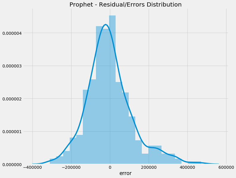 Example of a density curve from a previous blog post
Normal Distributions and its variations
Normal distributions (also known as Gaussian distributions) are the most common form of distribution for PDFs (i.e. continuous values). It is somewhat of a natural phenomenon - e.g. the height of people, the weight of birds etc.
It is also known as the bell curve. Generally speaking, normal distributions have the following characteristics:
- are symmetrical about the mean
- around 68% of the data points are within 1 standard deviation from the mean
 Image By M. W. Toews, CC BY 2.5, via Wikimedia Commons
However, in the real world, often the ideal normal/standard distribution doesn’t fit neatly. Therefore, we have variations on the normal distribution.
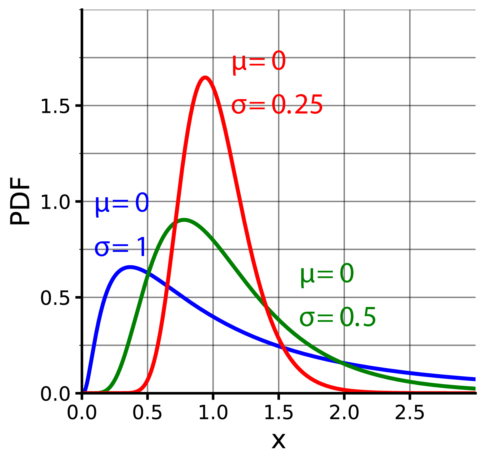
Lognormal Distribution and Exponential Modified Gaussian Distribution
A variation of the normal distribution is the lognormal distribution and Exponential Modified Gaussian Distribution.
These are similiar to the normal distribution, except that:
- curves are skewered to the right (i.e. longer tail on the right)
- curves are not symmetrical
- it includes a logrithmatic (lognormal) or exponential (EMG) component
 Xenonoxid, CC BY-SA 4.0, via Wikimedia Commons
Generalised Normal Distribution
When a variable doesn’t neatly fit into the ‘bell curve’ shape (e.g. it may be skewered), we can use a variation called the Generalised Normal Distribution.
A generalisation of a distribution means a variation of a distribution that fits better into real life scenarios (e.g. may include an exponential component).
To understand the how generalisation works, first we’ll discuss parametric vs nonparametric methods of modelling.
A parametric approach to modelling means the algorithm only gets a smaller sample of the data, and makes an assumption of what the data should fit into (e.g. normal distribution).
It is called parametric because using these assumptions, it tries to come up with the parameters that are fixed in advance (e.g. if it is a normal distribution, it tries to figure out the mean, standard deviation). It doesn’t tweak any additional parameters outside of the standard model.
In contrast, nonparametric methods don’t make any underlying assumption and try to come up with a function that best describes (i.e. generalises) the data. To do this, it looks at a much larger subset of the dataset. It will then add some shape parameters that tweak the overall shape/distribution (e.g. an exponential component).
Generalised normal distributions don’t have a specific form and come in all shapes and sizes - making it very powerful in describing many types of real-world datasets.
Logistic and Generalised Logistic Distributions
Logistic Functions and Generalised Logistic Distributions are similar to a Gaussian/normal distribution, but is designed more to fit variables with many extremes/outliers (e.g. rainfall modelling, where some days have very heavy rainfall).
The main difference between logistic vs normal distributions is logistic distributions penalise outliers more and have slightly heavier and longer tails compared to Gaussian/normal distributions.
 You can see above that logistic distributions generally have longer tails on the right-hand side
Image By Krishnavedala, CC0, via Wikimedia Commons
You can see above that logistic distributions generally have longer tails on the right-hand side
Image By Krishnavedala, CC0, via Wikimedia Commons
Gamma Distributions and its variations
Gamma Distributions are distributions which model things that always have positive values and have skewered distributions.
 As shown above, poisson distribution density curves with different lambdas
Gamma_distribution_pdf.png: MarkSweep and Cburnettderivative work: Autopilot, CC BY-SA 3.0, via Wikimedia Commons
As shown above, poisson distribution density curves with different lambdas
Gamma_distribution_pdf.png: MarkSweep and Cburnettderivative work: Autopilot, CC BY-SA 3.0, via Wikimedia Commons
Poisson/Exponential Distribution
A poisson distribution is special type of gamma distribution used to predict waiting times. It describes situations where:
- events occur at random points of time
- Each event is independent and does not influence the outcome of another event (i.e. it is a memoryless process)
- probability of success in an interval approaches zero as the interval becomes smaller
The lambda of the distribution determines the rate at which an event occurs (i.e. average number of events per time unit). The x-axis is generally time.
For example, if a bookshop gets on average 500 customers every night, what’s the probability that 1,000 customers will come next Friday night?
 As shown above, poisson distribution density curves with different lambdas
Image By Newystats, CC BY-SA 4.0, via Wikimedia Commons
As shown above, poisson distribution density curves with different lambdas
Image By Newystats, CC BY-SA 4.0, via Wikimedia Commons
For example, in the graph above, the blue curve (i.e. lambda = 1.5) means there’s around ~30% chance of the event occurring after 1 minute and basically 0% chance of the event occurring after 5 minutes.
Chi-squared Distribution
A Chi-squared distribution is a special type of gamma distribution that models the relationship between the theoretical/assumed version (i.e. expected) of the data vs the actual data (i.e. observed). It describes how ‘close’ a theoretical dataset is to the actual dataset.
The main parameter is the degrees of freedom (DF), which essentially is the number of observations the distribution has (generally speaking it is row count minus 1). The idea is the DF represents how many ‘independent’ data points you have.
The higher the degrees of freedom, the less skewered and more symmetrical the distribution will be.
 Higher Degrees of Freedom (k) means less skewered curves
Geek3, CC BY 3.0, via Wikimedia Commons
Higher Degrees of Freedom (k) means less skewered curves
Geek3, CC BY 3.0, via Wikimedia Commons
Empirical Cumulative Distribution Function
An empirical cumulative distribution function (ECDF) is basically the accumulated probability of a PD, so eventually it becomes 100%. ECDFs are equally applicable to both discrete and continuous variables. It is ‘empirical’ in the sense it is calculated based on the actual values of the variable.
The ECDF captures the characteristics of the whole field as it is distributed across the entire dataset. That is, it captures:
- Multi-modal areas - i.e. where the distribution has two or more ‘humps’
- Significant group of outliers. Unlike histograms, it is not dependent on the bins selected
- data skew - i.e. when the data isn’t normally distributed
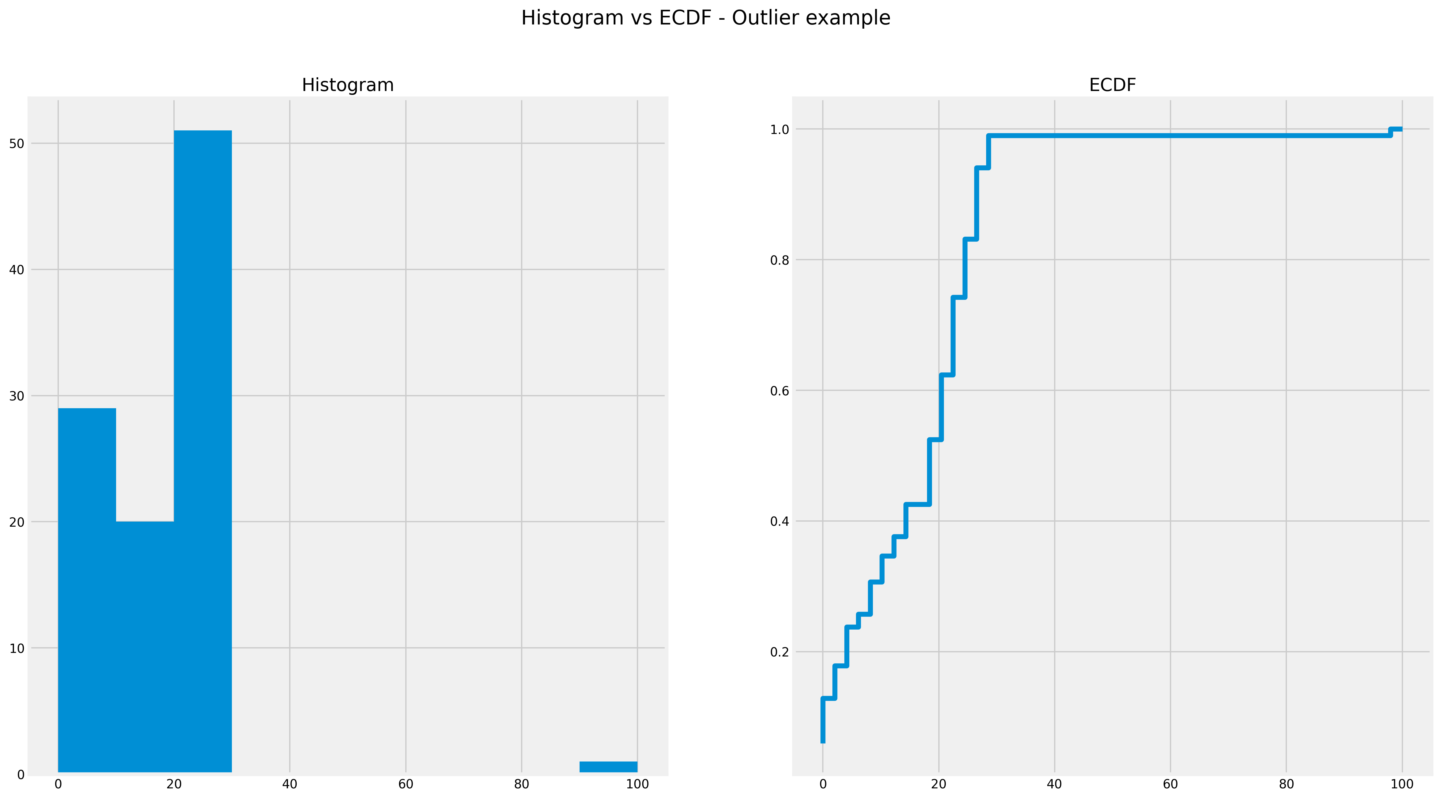 In the above ECDF, you can see that around 80% of the dataset is less than 20. You can also see that histograms don’t do a particularly good job of showing outliers.
ECDF with an Outlier
In the above ECDF, you can see that around 80% of the dataset is less than 20. You can also see that histograms don’t do a particularly good job of showing outliers.
ECDF with an Outlier
Essentially, it is good at retaining the ‘shape’ of the underlying data - as you can take just the ECDF and generate a dataset that will look very similar to the original dataset (albeit with a different scale).
Below you can see ECDF captures multiple ‘humps’ in one plot:
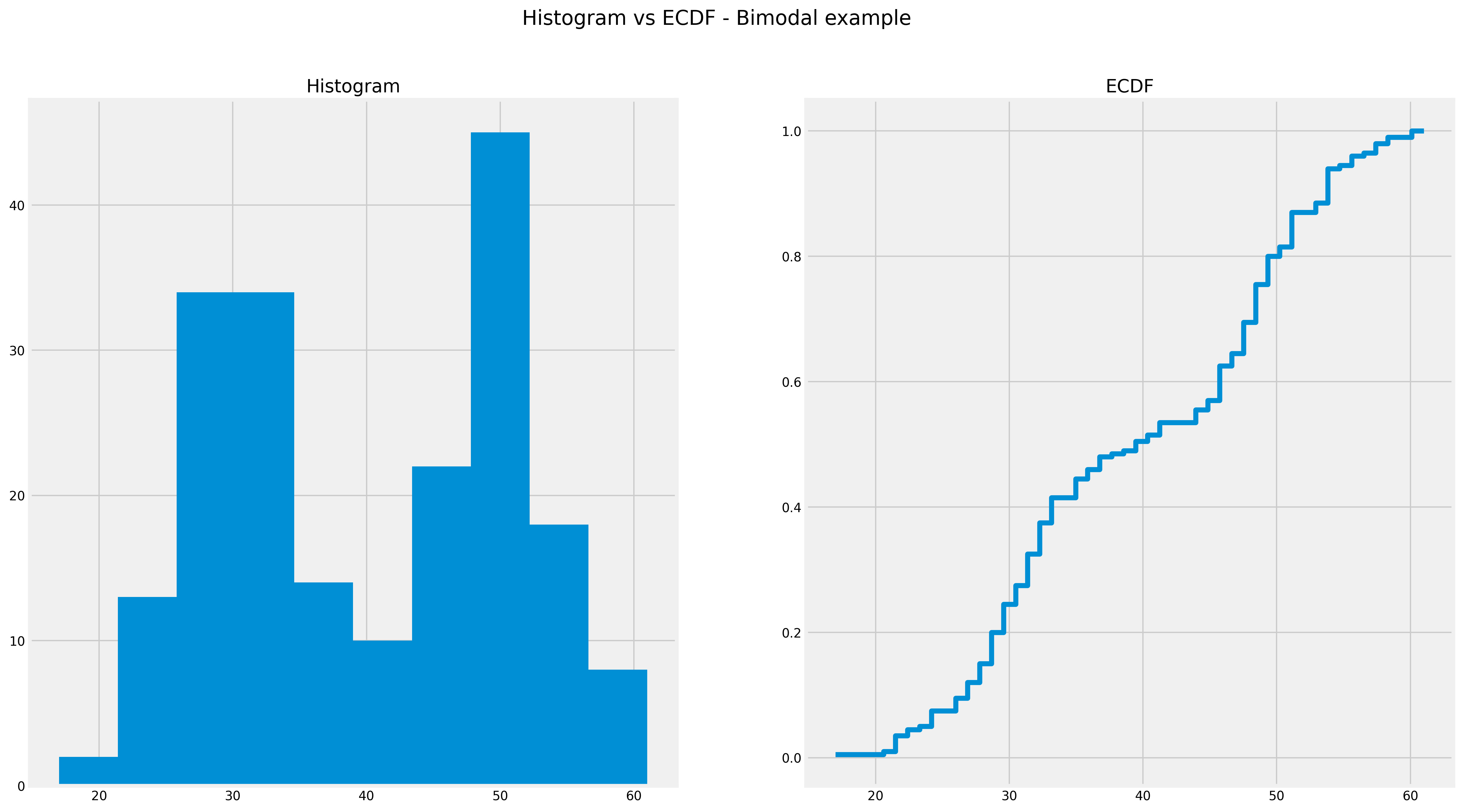 ECDF with multi-modal
Correlation
The correlation (i.e. Pearson’s R method) between two variables describes it’s relationship. Using this statistical measure, you can capture relationships between fields - e.g. if sale of cookies goes up, sale of milk goes up too.
The correlation is represented by a number between -100 to 100% (or -1 to 1). -100% represents a perfect inverse relationship (i.e. if X goes up, Y will go down) and 100% represents a perfect parallel relationship (i.e. if X goes up, Y will go up). 0% means no correlation between the two variables.
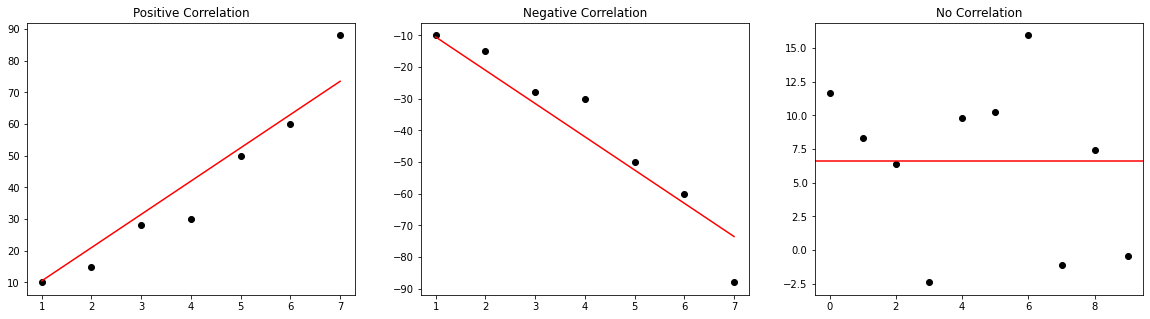 Correlations
Joint Multivariate Probability Distribution
Joint Probability Distribution is the PD when you look at 2 or more variables at a time - i.e. the probability of two events happening together. That is, PD you look at the distribution of one variable, but joint PD you look at multiple variables.
 Joint Probability Distribution visualistaion - you can see there’s multiple axes
IkamusumeFan, CC BY-SA 3.0, via Wikimedia Commons
Joint Probability Distribution visualistaion - you can see there’s multiple axes
IkamusumeFan, CC BY-SA 3.0, via Wikimedia Commons
If you fail to consider the joint PD, the statistical characteristics between features will be lost. For example, the real dataset shows higher income earners have a lower chance of having children.
If you only generate synthetic values based on the PD of income and cars alone (without considering the joint PD), you could end up with higher income earners have a higher chance of having children.
A common joint PD is a Gaussian Copula cumulative distribution function - the actual mathematics is very complicated (and you can read yourself), but the purposes of data work, you can calculate this using statsmodel off the correlation matrix (describe in the above section).
Another method is using Gaussian Mixture Models - it basically generates a bunch of gaussian/normal distributions that describe fit all the variables. It works similiarly to K-Means Clustering, in the sense it tries to group the variables into different clusters, with each cluster basically being a Gaussian distribution. The clusters’ relationships are also taken into account as well.
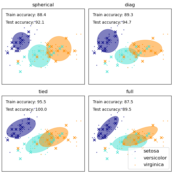 You can see the 4 attempts to cluster the data
From Scikit Learn official documentation
You can see the 4 attempts to cluster the data
From Scikit Learn official documentation
Now that we’ve done a recap of some statistical measures, next let’s discuss the methods in which to synthesis data.
Categorical Fields
To generate synthetic data for categorical fields, we generally use the normalised probability distribution. Normalised probability function does not equal normal distribution: normalised means all the values are scaled so it is between 0 to 1. That is, how many times did a value occur normalised as a % (i.e. relative frequencies)?
For example, let’s look at a categorical field and generate synthetic data:
import numpy as np
from faker import Faker

fake_data = Faker()

# First get the normalised probability of the 'city' field
dist = my_data['city'].value_counts(normalize=True)

# Generate fake names for the cities
cities = [fake_data.city() for x in range(5)]
# Create sample of 10,000 using the probability and fake cities
my_data['city'] = np.random.choice(
    a=cities, # the indices are the categories
    size=10000,
    p=dist
)
Another way is to retain the original values, but change the identifiers around. That is, the original statistical characteristics are kept, but are no longer associated with the original identifier:
# Like before, obtain the normalized probability dist
dist = my_data['car_brand'].value_counts(normalize=True)
# Randomly sample from the dist and replace the existing values
my_data['car_brand'] = np.random.choice(
    a= dist.index,
    p=dist,
    size=len(my_data)
)
Continuous Data
For continuous data, we generally use a PDF that best captures the data (e.g. normal distribution, exponential etc.). To do this, we basically fit the different types of distributions into the dataset and see which one has the best fit (using a goodness-of-fit metric or error-based metric, such as sum of squared errors).
In the below example, we will use an open-source library Fitter to assist us with finding the best fit.
from fitter import Fitter

# Backend of Fitter is Scipy
# Fitter will fit dataset against specified distributions
# and rank based on sum of squared errors (SSE)
dists = [
  'norm', # Normal
  'lognorm', # Lognormal
  'exponnorm', # Exponentially modified normal
  'gamma', # Gamma
  'chi2', # Chi-Squared
  'expon', # Exponential
  'genlogistic', # Generalised Logistic
  'gennorm', # Generalised Normal
  'genexpon' # Generalised Exponential
]

f = Fitter(
    data,
    distributions=dists
)

f.fit()
f.get_best(method='sumsquare_error')

# In the above, our experiment concluded that
# generalised normal distribution was the best it
from scipy.stats import gennorm

model.fit(data['salaries'])
# Fit the distribution
params = gennorm.fit(data['salaries'])

# Sample (i.e. randomly generate) from
# the distribution and replace salaries
data['salaries'] = norm.rvs(
    size=len(data.index),
    *params
)
A drawback of doing both these approaches is that all the interactions or correlations between the variables might be lost. For example, in an original dataset, women had a higher writing score than men. In the generated dataset, this relationship may no longer exist.
The above examples you will notice fail to take into account correlation and joint probability distribution. Without the use of neural networks, it is very difficult to do this.
Using Open-source Libraries for Synthetic Data Generation
Fortunately, there are great open-source libraries out there that harness neural networks to generate synthetic data. In particular, Synthetic Data Vault (SDV)’s CTGAN model uses a generative adversrial network (GAN) to generate high-quality sythentic data.
It does this by pitting two competing neural networks - a generator which tries to create synthetic data that matches the real data as much as possible vs. discriminator, which tries to distinguish between real data vs synthetic data.
In addition, SDV uses other complex probabilistic graphical modelling and neural network techniques (e.g. hierarchical generative modelling and recursive sampling). This allows the GAN to preserve:
-
Probability distributions within a variable
-
Multi-modal distributions for variables
-
Joint multivariate probability distributions between variables
-
Correlations between variables
The result is a pretty decent synthetic data generator!
It is surprisingly simple to use. For example:
from sdv.tabular import CTGAN

# Fit the GAN model
model = CTGAN()
model.fit(my_data)

# Sample 2000 synthetic data records
synthetic_data = model.sample(2000)
Conclusion
As data privacy becomes even more important, incorporating it into our day-to-day data work is a must-have (and no longer a nice-to-have). Hopefully this blog gives you a bit of flavour in some ways to comply with data privacy rules!
 Image By Pixabay